 Lapsed, fee not paid11 drawings
Software & Apps · US 9,946,807 B2
System, method and computer program product for providing content based upon a representation of the same
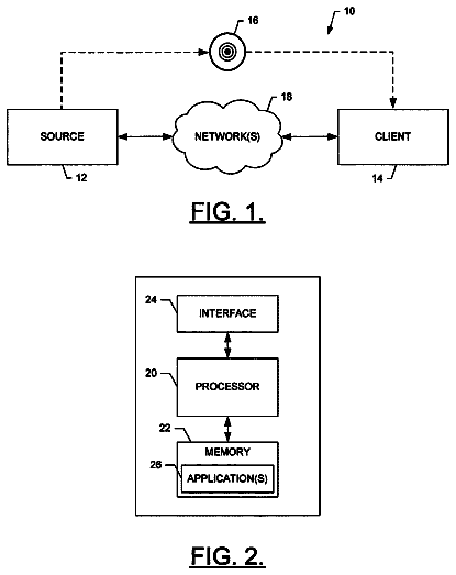
A system for providing content includes a source and a client.
US 9,946,817 B2 · Assignee: SUMITOMO RUBBER INDUSTRIES, LTD. · Inventors: Ueno; Shinichi
Sheet 1 of 9 from the published document. All sheets in the USPTO PDF
A method for calculating an interaction potential between filler particles in a polymeric material by using a computer is disclosed. The method comprises: arranging filler models and polymer models in a virtual space; calculating a free energy in the virtual space based on a mean field theory; obtaining parameters of the Lennard-Jones potential by approximating the free energy to the Lennard-Jones potential.
The present invention relates to a method for calculating an interaction potential between filler particles in a polymeric material, more particularly to a method for determining parameters of the Lennard-Jones potential between the filler particles. In recent years, in order to develop or design rubber compositions, various computer simulation methods for evaluating properties of a composite of a polymeric material and filler have been proposed. In such a simulation method, for example, filler models of filler particles are defined, and the Lennard-Jones potential U.sub.LJ given by the following equation (namely, an interaction potential between two filler models) is defined between the filler models. U LJ ( r ij ) = 4 .Math. LJ { ( σ LJ r ij ) 12 - ( σ LJ r ij ) 6 } Equation ( 1 ) wherein r.sub.ij is the distance between two filler models, ϵ.sub.LJ is a coefficient for the in
1 of 9 drawing sheets so far from the published document, cropped to the drawing. Every sheet is in the USPTO PDF.
What the patent claimed, word for word. All of it is now free to use.
The present invention relates to a method for calculating an interaction potential between filler particles in a polymeric material, more particularly to a method for determining parameters of the Lennard-Jones potential between the filler particles.
In recent years, in order to develop or design rubber compositions, various computer simulation methods for evaluating properties of a composite of a polymeric material and filler have been proposed.
In such a simulation method, for example, filler models of filler particles are defined, and the Lennard-Jones potential U.sub.LJ given by the following equation
(namely, an interaction potential between two filler models) is defined between the filler models.
U LJ ( r ij ) = 4 .Math. LJ { ( σ LJ r ij ) 12 - ( σ LJ r ij ) 6 } Equation ( 1 ) wherein r.sub.ij is the distance between two filler models, ϵ.sub.LJ is a coefficient for the intensity of the potential between the filler models, and σ.sub.LJ corresponds to the diameter of the filler models.
Heretofore, the above-mentioned parameters σ.sub.LJ and ϵ.sub.LJ have been determined by an operator based on his/her intuition and experience, therefore, it is difficult to perform the simulation with high accuracy.
It is therefore, an object of the present invention to provide a method for calculating an interaction potential between filler particles in a polymeric material, by which parameters of the interaction potential, in particular, the Lennard-Jones potential between the filler particles can be determined by the use of a computer though a calculation.
According to the present invention, a method for calculating an interaction potential between filler particles in a polymeric material by using a computer, comprises:
a process in which a filler model of each of the filler particles is defined,
a process in which a polymer model of each of macromolecular chains of the polymeric material is defined,
a process in which the filler models and the polymer models are set in a predetermined virtual space,
a process in which a free energy in the virtual space is calculated based on the mean field theory, and
a process in which, by approximating the free energy to the Lennard-Jones potential, parameters of the Lennard-Jones potential are obtained.
In the present invention, therefore, the parameters of the Lennard-Jones potential can be determined based on the free energy in the virtual space. This is based on findings of the present inventor obtained through experiments, namely, the free energy in the virtual space calculated based on the mean field theory approximates the interaction potential between the filler models. Thus, the parameters can be determined without the need for human intuition and experience. As a result, it is possible to perform the simulation with high accuracy.
The calculating method according to the present invention may further include the following features (1)-(3):
the filler models are a pair of the filler models, and the process for calculating the free energy comprises
a step (a) in which, by abutting the filler models, a minimum value Es of the free energy is calculated, and
a step (b) in which, by separating the filler models from each other, a maximum value Fm of the free energy is calculated;
the filler models have a certain diameter, and the parameters of the Lennard-Jones potential include
a parameter ϵ.sub.LJ relating to the strength of a repulsive force exerted between the filler models by the Lennard-Jones potential, and
a parameter σ.sub.LJ corresponding to the diameter of the filler models, and
the process for obtaining the parameter ϵ.sub.LJ and parameter σ.sub.LJ comprises
a step (c) in which the parameter ϵ.sub.LJ is obtained from the difference between the maximum value Fm and the minimum value Fs of the free energy, and
a step (d) in which the parameter σ.sub.LJ is obtained from a distance between the filler models which abut each other to calculate the minimum value Fs of the free energy;
a χ parameter relating to an interaction between a filler model and a polymer model is set in a range of from 0.0 to 10.0.
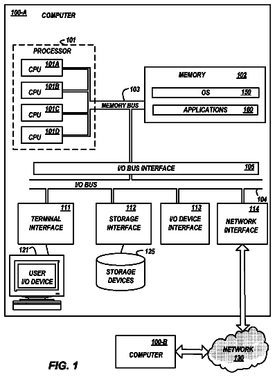
FIG. 1 shows a computer for implementing a method for calculating an interaction potential between filler particles in a polymeric material according to the present invention.
FIG. 2 is a flow chart of the calculating method according to the present invention.
FIG. 3 is a diagram showing a virtual space used to obtain parameters of the Lennard-Jones potential.
FIG. 4 is a diagram showing a filler model and polymer models.
FIG. 5 is a diagram showing the filler models and the polymer models arranged in the virtual space.
FIG. 6 is a flow chart of a simulation process of the calculating method.
FIGS. 7( a ) and 7( b ) are diagrams showing the filler models in the virtual space for explaining processes for obtaining the minimum value Fs and the maximum value Fm of the free energy F in the virtual space.
FIG. 8 is a graph showing a relationship between the free energy in the virtual space and the distance between the filler models.
FIG. 9 is a diagram showing a virtual space used to perform a deformation calculation by defining the Lennard-Jones potential on filler models set in the virtual space.
FIG. 10 is a graph showing a relationship between the Lennard-Jones potential and the distance between the filler models.
FIG. 11 is a flow chart of a calculation process of the calculating method.
Embodiments of the present invention will now be described in detail in conjunction with the accompanying drawings.
The method for calculating an interaction potential between filler particles in a polymeric material according to the present invention (abbreviated to “calculating method”) is carried out by the use of a computer 1 .
Here, the filler may be any kind of filler including carbon black, silica, alumina and the like. The polymeric material may be any kind of polymer including rubber, elastomer, resin and the like.
As shown in FIG. 1 for example, the computer 1 implementing the calculating method comprises a main body 1 a , a keyboard 1 b , a mouse 1 c and a display 1 d . The main body 1 a comprises an arithmetic processing unit (CPU), memory, storage devices such as magnetic disk, disk drives 1 a 1 and 1 a 2 and the like. In the storage device, programs/software for carrying out the calculating method is stored.
FIG. 2 shows a flow chart of the calculating method as an embodiment of the present invention. The entire process thereof will be explained hereunder.
* Process S 1
In the process S 1 , a virtual space 3 is defined. In this embodiment, as shown in FIG. 3 , the virtual space 3 is two-dimensional and has a horizontally long rectangular shape. on the respective sides 3 a and 3 b surrounding the virtual space 3 , periodic boundary conditions are defined.
The length L1 of the sides 3 a and the length L2 of the sides 3 b may be set arbitrarily, but it is preferable that the length L1 and the length L2 are set in a range of not less than 2 times, more preferably not less than 10 times the radius of gyration of the filler models 4 and the polymer model 6 (shown in FIG. 4 ). Data about such virtual space 3 are stored in the computer 1 . * Process S 2
In the process S 2 , a filler model of each of the filler particles is defined.
As shown in FIG. 4 , the filler model 4 is defined by a single filler segment 4 s forcibly set in one domain 5 of the virtual space 3 divided into particles or a mesh. Namely, the filler segment 4 s is constrained to the domain 5 .
In this embodiment, the domain 5 is two-dimensional and defined as being of a circular shape. However, in the case of a three-dimensional filler model 4 where the filler segment 4 s is also three-dimensional, it is preferable that the domain 5 is defined as being of a spherical shape. In any case, data about the filler model 4 are stored in the computer 1 .
In this embodiment, the filler segment 4 s is treated as a minimum unit of a simulation based on the mean field theory (Flory-Huggins theory, etc.). Here, the mean field theory is a statistical thermodynamic theory for polymer solution used to mean-field approximate the interactions between a polymer and its surroundings.
* Process S 3
In the process S 3 , a polymer model of each of macromolecular chains of the polymeric material is defined. As shown in FIG. 4 , the polymer model 6 is defined by a plurality of polymer segments 7 . As with the filler segment 4 S, the polymer segment 7 is treated as a minimum unit of a simulation based on the mean field theory.
Between the polymer segments 7 , a joining chain 8 is defined. For example, the length K1 of the joining chain 8 is set to a value corresponding to the mesh size of the system. Thus, the polymer model 6 is defined to have a two-dimensional straight-chain structure in which the relative distances between the polymer segments 7 are held stably.
A χ parameter K2 employed in the Flory-Huggins theory and relating to an interaction between a polymer segment 7 of a polymer model 6 and a polymer segment 7 of another polymer model 6 is set in a range of from 0.0 to 10.0 for example. As a result, between the polymer segments 7 , a repulsive interaction and the intensity thereof are defined. Data about such the polymer segments 7 are stored in the computer 1 .
* Process S 4
In the process S 4 , the filler models 4 and the polymer models 6 are set in the virtual space 3 to have a predetermined volume fraction. For example, the volume fraction is set in a range of from 50% to 99%. In this embodiment, a pair of the filler models are set in the virtual space 3 . Data about the concentration distribution of the polymer segments 7 of the polymer models 6 are stored in the computer 1 .
* Process S 5
In the process S 5 , a χ parameter K3 employed in the Flory-Huggins theory and relating to an interaction between a filler model 4 and a polymer model 6 is defined.
As shown in FIG. 4 , χ parameters K3 are defined between the filler segments 4 S and the polymer segments 7 .
In this embodiment, the χ parameters K3 are set in a range of from 0.0 to 10.0. As a result, between the filler segment 4 S and the polymer segment 7 , a repulsive interaction and the intensity thereof are defined.
If the χ parameters K3 are more than 10.0, there is a possibility that, in the simulation based on the mean field theory, even if the arrangement of the filler models 4 and the polymer models 6 becomes close to their equilibrium state, the difference in the calculated energy from that calculated in the most recent calculation step is still large, and the computation can not be converged. Therefore, preferably, the χ parameters K3 are set in a range of not more than 5.0. Such χ parameters K3 are stored in the computer 1 . * Simulation Process S 6
In the simulation process S 6 , using the filler models 4 and the polymer models 6 set in the virtual space 3 , a free energy in the virtual space 3 is calculated based on the mean field theory. Here, the free energy F is the Helmholtz free energy.
As shown in FIG. 5 , in the simulation based on the mean field theory, the free energy F of the equilibrium state of the virtual space including the filler models 4 and the polymer models 6 , is calculated based on the SCF method (Self-Consistent Field Method) taking into account the entropy of the arrangement of the polymer models 6 .
Such simulation based on the mean field theory can be implemented, for example, by the use of a simulation engine SUSHI built in a simulation system OCTA available from a website.
FIG. 6 shows a flow chart of the simulation process S 6 .
** Process S 61
In the process S 61 , by abutting the filler models 4 , a minimum value Fs of the free energy F is calculated.
As shown in FIG. 7( a ) , a pair of the filler models 4 are abutted each other, and the free energy F in the virtual space 3 under such abutting state of the pair of the filler models 4 is calculated.
In the abutting state of the pair of the filler models 4 , the number of the polymer models 6 entering into the vicinity of the filler models 4 becomes least.
Therefore, a reduction in the entropy of the arrangement of the polymer models 6 is suppressed, and the free energy F in the virtual space 3 becomes a minimum value Fs.
In FIG. 7( a ) and FIG. 7( b ) , the polymer models 6 (shown in FIG. 5 ) are omitted for convenience sake.
Further, in the process S 61 , a distance R between the filler models 4 abutting each other, namely, the minimum distance Rs is obtained.
Here, the distance R between the filler models 4 is defined as the distance between the centers (centroids) 5 c of the domains in which the filler segment 5 are disposed.
The obtained minimum value Fs of the free energy F and the obtained minimum distance Rs are stored in the computer 1 .
** Process S 62
In the process S 62 , by separating the abutting filler models 4 from each other, a maximum value Fm of the free energy F is calculated.
As shown in FIG. 7( b ) , while the distance R is gradually increased, the free energy F in the virtual space 3 is calculated.
The distances R and the free energy F of the entire system calculated at each distance R are stored in the computer 1 . Thus, a relationship between the free energy F and the distance R can be obtained as shown in FIG. 8 . As shown, with the increase in the distance R, the number of polymer models 6 entering into the vicinity of the filler models 4 is increased, and the free energy F in the virtual space 3 is increased. In this embodiment, the distance R between the filler models 4 is increased until the increment of the free energy becomes substantially zero to thereby obtain the maximum value Fm of the free energy F.
* Calculation Process S 7
In the calculation process S 7 , by approximating the free energy F to the Lennard-Jones potential U.sub.LJ, parameters of the Lennard-Jones potential U.sub.LJ are obtained by the computer 1 . The Lennard-Jones potential U.sub.LJ is given by the following equation (1).
U LJ ( r ij ) = 4 .Math. LJ { ( σ LJ r ij ) 12 - ( σ LJ r ij ) 6 } Equation ( 1 ) wherein r.sub.ij is the distance between two filler models, ϵ.sub.LJ is a coefficient for the intensity of the potential between the filler models, and σ.sub.LJ corresponds to the diameter of the filler models. Here, the distance r.sub.ij is the distance between the centers of the filler models. In a molecular dynamics calculation, such Lennard-Jones potential U.sub.LJ is able to define a repulsive force acting between the filler models.
FIG. 10 is a graph showing a relationship between the Lennard-Jones potential U.sub.LJ and the distance r.sub.ij.
when the distance r.sub.ij is 2.sup.1/6σ.sub.LJ, the Lennard-Jones potential U.sub.LJ becomes a minimum value −ϵ.sub.LJ.
when the pair of the filler models abut each other, the Lennard-Jones potential U.sub.LJ becomes minimized.
Accordingly, the distance r.sub.ij when the pair of the filler models abut each other is 2.sup.1/6σ.sub.LJ.
when the distance r.sub.ij is decreased toward zero from 2.sup.1/6σ.sub.LJ, the Lennard-Jones potential U.sub.LJ increases to infinity and exerts a large repulsive force between the filler models.
when the distance r.sub.ij is increased from 2.sup.1/6σ.sub.LJ, the Lennard-Jones potential U.sub.LJ gradually decreases and approaches to zero. This means that the influence of the Lennard-Jones potential U.sub.LJ is reduced with the increase in the distance r.sub.ij.
The inventor found that, as a result of the above facts correlated, there is a correlation between the free energy F and the Lennard-Jones potential U.sub.LJ.
In the present invention, by making a calculation based on the free energy F which varies according to the distance R, the parameters σ.sub.LJ and ϵ.sub.LJ of the Lennard-Jones potential U.sub.LJ is determined without the need for someone's intuition and experience.
FIG. 11 shows a flow chart of the calculation process S 7 for obtaining the parameters σ.sub.LJ and ϵ.sub.LJ.
** Process S 71
In the process S 71 , the parameter ϵ.sub.LJ is obtained from the difference (Fm−Fs) between the maximum value Fm and the minimum value Fs of the free energy.
As shown in FIG. 10 , when the distance r.sub.ij is in the range from 2.sup.1/6σ.sub.LJ to the higher, the difference between the maximum Lennard-Jones potential U.sub.LJ
and the minimum Lennard-Jones potential U.sub.LJ (−ϵ.sub.LJ) is ϵ.sub.LJ.
In the process S 71 , this difference (ϵ.sub.LJ) is regarded as the same value as the difference (Fm−Fs).
Namely, ϵ.sub.LJ =Fm−Fs Expression (2). Using this relational expression (2), the parameter ϵ.sub.LJ is obtained. The obtained parameter ϵ.sub.LJ is stored in the computer 1 . ** Process S 72
In the process S 72 , the parameter σ.sub.LJ is obtained from a distance between the filler models abutting each other.
As shown in FIG. 10 , in the Lennard-Jones potential U.sub.LJ, the distance r.sub.ij between the abutting filler models is 2.sup.1/6σ.sub.LJ.
In the process S 72 , this distance r.sub.ij (2.sup.1/6σ.sub.LJ) is regarded as the same value as the minimum distance Rs.
Namely, 2.sup.1/6σ.sub.LJ =Rs. Accordingly, σ.sub.LJ =Rs/ 2.sup.1/6 Expression (3). using this relational expression (3), the parameter σ.sub.LJ is obtained. The obtained parameter σ.sub.LJ is stored in the computer 1 .
In the process S 7 , therefore, the parameters ϵ.sub.LJ and σ.sub.LJ of the Lennard-Jones potential can be obtained by the calculation based on the free energy F in the virtual space including the filler models as the analysis object. Thus, depending on the analysis object (filler models), the parameters ϵ.sub.LJ and σ.sub.LJ suitable for the analysis object can be obtained without the need for someone's intuition and experience, therefore, it is possible to perform the simulation with high accuracy.
* Process S 8
In the process S 8 , a virtual space 13 including filler models 11 and polymer models 14 and corresponding to a micro-structural part of the polymeric material as the analysis object is newly defined, and
a deformation calculation of the virtual space 13 is performed.
In this embodiment, as shown in FIG. 9 , the virtual space 13 is defined as a cube having three pairs of parallelly-opposed wall surfaces 13 s . on each of the wall surfaces 13 s , periodic boundary conditions are defined.
The filler models 11 are each defined by a single filler particle model 12 having a spherical shape and treated as a mass point of the equation of motion.
Between the filler models 11 , there is defined the Lennard-Jones potential U.sub.LJ given by the above-mentioned equation
to which the values of the parameters ϵ.sub.LJ and σ.sub.LJ obtained in the above-mentioned process S 7 are assigned.
The polymer models 14 which are of macromolecular chains of the polymeric material, are defined as a uniform fluid existing in the virtual space 13 between the filler models 11 and the wall surfaces 13 s . on the polymer models 14 , the viscosity of the polymeric material is defined.
Data about such virtual space 13 including the filler models 11 and the polymer models 14 are stored in the computer 1 .
Then, the deformation calculation of the virtual space 13 is performed based on the Navier-stokes equation and the motion equation.
In this embodiment, the deformation calculation is performed until the strain becomes a value in a range of from 1 to 100, and a physical property (for example, viscosity, stress etc.) of the virtual space 13 is calculated.
The deformation rate of the virtual space 13 is set in a range of from about 10.sup.−6 to 1 σ/τ.
On the assumption that the filler models 11 follow the classical dynamics, the Newton's equation of motion is employed.
The motions of the filler models 11 are tracked at regular time intervals.
During the deformation calculation, the number of the filler models in the virtual space, and the temperature and the volume of the virtual space are kept constant.
For example, such deformation calculation can be implemented by the use of a simulation software KAPSEL available from the same website as the above-mentioned simulation system OCTA.
As explained above, in the process S 8 , the parameters ϵ.sub.LJ and σ.sub.LJ of the Lennard-Jones potential U.sub.LJ are set to the values of the parameters ϵ.sub.LJ and σ.sub.LJ obtained by the calculation process S 7 .
* Process S 9
In the process S 9 , the computer 1 judges whether the physical property of the virtual space 13 is acceptable or not.
If not acceptable, the conditions of the filler models 11 and the polymer models 14 are changed.—Process S 11
Then, the processes S 1 to S 9 are repeated.
If acceptable, based on the conditions of the filler models 11 and the polymer models 14 , the polymeric material including the filler is actually produced.—Process S 10
Thus, in this embodiment, the conditions of the filler models 11 and the polymer models 14 are changed until the physical property of the virtual space 13 becomes acceptable, therefore, the polymeric material with desired performance can be developed efficiently.
Confirmation Test
According to the procedure shown in FIG. 2 , the parameters ϵ.sub.LJ and σ.sub.LJ were obtained, and the deformation calculation of the virtual space was performed in order to obtain the viscosity of the polymeric material including the filler. The obtained viscosity was compared with the actual measurement value. As a result, it was confirmed that the obtained viscosity well corresponds to the actual measurement value. The conditions and parameters used in the calculations are as follows.
In the process for obtaining the parameters ϵLJ and αLJ, virtual space 3 :
L1: 30 σ
L2: 60 σ
Filler Model 4 :
Number in the virtual space: 2
Diameter: 6 σ
Polymer Model 6 :
volume fraction in the virtual space: 80%
Chain length of polymer segment: 50 (Linear molecule)
Diameter of polymer segment: 1 σ
χ parameter K2 between polymer models: 0.0
χ parameter K3 between filler model and polymer model: 3.0.
In the deformation calculation,
virtual space 13 : cube
L1 of each side: 300 σ
Filler model 11 :
Number in the virtual space: 100
Diameter: 6 σ
Polymer model 14 :
Viscosity: 1.0 η
Absolute temperature: 1.0ϵ/kB.
About 3,907 words. The USPTO PDF has it with every drawing.
Fees are due 3.5, 7.5 and 11.5 years after grant. This patent expired on April 17, 2026, so the fee marked "not paid" was the one that went unpaid.
METHOD FOR CALCULATING INTERACTION POTENTIAL BETWEEN FILLER PARTICLES IN POLYMERIC MATERIAL
Filed Jun 2014 · published Dec 2014Method for calculating interaction potential between filler particles in polymeric material
Filed Jun 2014 · granted Apr 2018Earlier publications, parents and continuations. None of them can still be enforced, or this patent would not be listed.
Prior art cited by the examiner or applicant. Useful when you check your own idea for novelty.
Everything on this page comes from the documents linked above.