 Lapsed, fee not paid12 drawings
Industrial Equipment · US 9,823,191 B2
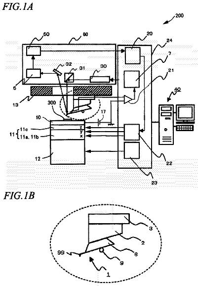
Micro-prism test chip
A disposable micro-prism test chip for surface plasmon resonance measurement comprises a micro-tray and a micro-prism mounted on the micro-tray.
US 9,823,205 B2 · Assignee: SCHLUMBERGER TECHNOLOGY CORPORATION · Inventors: Luo; Zhixiang et al.
Sheet 1 of 8 from the published document. All sheets in the USPTO PDF
Methods and systems for determining surface relaxivity from nuclear magnetic resonance measurements relate to applying multiple nuclear magnetic resonance (NMR) diffusion editing Carr-Purcell-Meiboom-Gill (CPMG) pulse sequences to the porous medium, wherein the diffusion editing CPMG pulse sequences have a diffusion encoding time Δ; receiving NMR data generated by the pulse sequences; processing the received NMR data to obtain a distribution f(T.sub.2,D) for the diffusion encoding time Δ; repeating the applying, the receiving, and the processing at least one time for pulse sequences having different respective diffusion encoding times Δ to obtain respective distributions f(T.sub.2,D) corresponding respectively to the different diffusion encoding times Δ; and utilizing the respectively obtained distributions f(T.sub.2,D) to generate a surface relaxivity (ρ) determination.
Nuclear magnetic resonance (NMR) is a useful tool in the determination of the pore size distribution (PSD) of a porous medium. The PSD of a medium can be determined by making relaxation measurements of a fluid saturating the medium. In particular, the T.sub.2 spin-spin relaxation time is related to pore size according to 1 T 2 = 1 T 2 b + ρ S V , where T.sub.2b is the T.sub.2 value of the bulk fluid, ρ is the surface relaxivity, and S/V is the surface volume ratio. See, e.g., Kleinberg, R., et al., “Utility of NMR T.sub.2 distributions, connection with capillary pressure, clay effect, and determination of the surface relaxivity parameter ρ.sub.2,” Magnetic Resonance Imaging, Vol. 14 pp. 761-767 (1996)). The determination of surface relaxivity ρ may be considered important for quantitative interpretation of NMR data. Surface relaxivity is usually determined by finding the value of ρ t
1 of 8 drawing sheets so far from the published document, cropped to the drawing. Every sheet is in the USPTO PDF.
What the patent claimed, word for word. All of it is now free to use.
Independent claims stand on their own. The others add detail to the claim they name.
The subject disclosure relates to the measurement of the properties of a medium such as rock. More particularly, the subject disclosure relates to methods for determining surface relaxivity of a medium using nuclear magnetic resonance. The subject disclosure has particular application to the hydrocarbon industry, although it is not limited thereto.
Nuclear magnetic resonance (NMR) is a useful tool in the determination of the pore size distribution (PSD) of a porous medium. The PSD of a medium can be determined by making relaxation measurements of a fluid saturating the medium. In particular, the T.sub.2 spin-spin relaxation time is related to pore size according to
1 T 2 = 1 T 2 b + ρ S V , where T.sub.2b is the T.sub.2 value of the bulk fluid, ρ is the surface relaxivity, and S/V is the surface volume ratio. See, e.g., Kleinberg, R., et al., “Utility of NMR T.sub.2 distributions, connection with capillary pressure, clay effect, and determination of the surface relaxivity parameter ρ.sub.2,” Magnetic Resonance Imaging, Vol. 14 pp. 761-767 (1996)). The determination of surface relaxivity ρ may be considered important for quantitative interpretation of NMR data. Surface relaxivity is usually determined by finding the value of ρ that matches the PSD derived from the NMR T.sub.2 distribution to the PSD of an independent laboratory measurement, for example via a capillary pressure measurement. See, e.g., Borgia, G., et al., “Nuclear magnetic resonance relaxivity and surface-to-volume ratio in porous media with a wide distribution of pore sizes,” Journal of Applied Physics, Vol. 79 pp. 3656-3664 (1996); and Basan, P. B., et al., “Pore-size data in petrophysics: a perspective on the measurement of pore geometry,” Geological Society, London, Special Publications, Vol. 122 pp. 47-67 (1997). However, an independent measurement of the surface area is not always available, such as in formation (borehole) logging applications where the medium remains in situ.
When water is located inside a porous medium, motion of the water is affected by the solid matrix of that medium. The corresponding effect on the apparent diffusion coefficient is well established both theoretically and experimentally and that effect may be utilized to probe the S/V information. See, Mitra, P. P., et al., “Diffusion propagator as a probe of the structure of porous media,” Physical Review Letters, Vol. 68 pp. 3555-3558 (1992); and Latour, L. L., et al., “Time-dependent diffusion coefficient of fluids in porous media as a probe of surface-to-volume ratio,” Journal of Magnetic Resonance, Series A, Vol. 101 pp. 342-346 (1993). Recently, a purely in-situ NMR logging approach that combines T.sub.2 relaxation and diffusion measurements to determine surface relaxivity was proposed. See, Zielinski, L., et al., “Restricted Diffusion Effects in Saturation Estimates from 2D Diffusion-Relaxation NMR Maps,” SPE Annual Technical Conference and Exhibition, 2010; and Zielinski, L., et al., “Method for Determining Rock Formation Fluid Interaction Properties Using Nuclear Magnetic Resonance Well Logging Measurements,” U.S. Patent Publication #2013/0057277
which is hereby incorporated by reference herein in its entirety. An apparent advantage of using restricted diffusion to determine S/V is that T.sub.2 relaxation is affected by paramagnetic centers on the surface through the diffusion process. See, Brownstein, K. R., and Tarr, C., “Importance of classicial diffusion in NMR studies of water in biological cells,” Physical Review A, Vol. 19 p. 2446 (1979); Wilkinson, D. J., et al., “Nuclear magnetic relaxation in porous media: The role of the mean lifetime τ(ρ,D),” Physical Review B, Vol. 44 p. 4960 (1991). Unlike systems that use one dimensional time dependent diffusion data to determine surface relaxivity, Zielinski et al. analyze a 2D diffusion-relaxation (DT.sub.2) map which contains S/V information as function of pore size instead of the ratio of total surface to total volume (S.sub.T/V.sub.T).
Zielinski et al.'s methodology is suitable to homogenous (e.g., single pore size length scale) sample applications where T.sub.2 differs notably from its bulk value. The methodology utilizes inputs to the analysis such as tortuosity, bulk diffusion coefficients, and a fixed heterogeneity length.
This summary is provided to introduce a selection of concepts that are further described below in the detailed description. This summary is not intended to identify key or essential features of the claimed subject matter, nor is it intended to be used as an aid in limiting the scope of the claimed subject matter.
In accordance with example embodiments, a method of determining surface relaxivity of a porous medium includes: applying multiple nuclear magnetic resonance (NMR) diffusion editing Carr-Purcell-Meiboom-Gill (CPMG) pulse sequences to the porous medium, wherein the diffusion editing CPMG pulse sequences have a diffusion encoding time Δ; receiving NMR data generated by the pulse sequences; processing the received NMR data to obtain a distribution f(T.sub.2,D) for the diffusion encoding time Δ; repeating the applying, the receiving, and the processing at least one time for pulse sequences having different respective diffusion encoding times Δ to obtain respective distributions f(T.sub.2,D) corresponding respectively to the different diffusion encoding times Δ; and utilizing the respectively obtained distributions f(T.sub.2,D) to generate a surface relaxivity (ρ) determination.
In accordance with example embodiments, a method of determining surface relaxivity of a porous medium includes: (a) generating multiple nuclear magnetic resonance (NMR) diffusion editing−CPMG (Carr-Purcell-Meiboom-Gill) pulse sequences with a diffusion encoding time Δ that interact with the porous medium, and acquiring resulting data; (b) processing the resulting data to obtain a distribution f(T.sub.2,D) for that Δ; (c) calculating a mean diffusion coefficient D (T.sub.2s) for each T.sub.2 value, where T.sub.2s is the transverse relaxation time due to surface relaxation; (d) calculating a T.sub.2 distribution g(T.sub.2s); (e) utilizing the calculated T.sub.2 distribution and the calculated mean diffusion coefficient in order to generate a determination of surface relaxivity (ρ) by choosing values for the surface relaxivity and at least one parameter to cause a fitting function of the surface relaxivity and a parameter Γ to closely approximate the average diffusion coefficient D (T.sub.2s), the fitting function is defined by
D ( Δ , T 2 s ) D 0 = 1 - ( 1 - α ) β L D ρ T 2 s + ( 1 - α ) ( L D Γ ρ T 2 s ) 2 ( 1 - α ) + β L D ρ T 2 s + ( 1 - α ) ( L D Γ ρ T 2 s ) 2 where D.sub.0 is a bulk diffusion coefficient,
D ( ∞ ) / D 0 , β = 4 9 π , L D = D 0 Δ , and Γ = L M / ρ T 2 s , where L.sub.M is a length scale characterizing a transition between a short-time and long-time diffusion limit.
In accordance with example embodiments, a method utilizing nuclear magnetic resonance (NMR) measurements to determine surface relaxivity of a porous medium includes: (a) generating multiple NMR diffusion editing pulse sequences for each of a plurality of diffusion encoding times Δ that interact with the porous medium, and acquiring resulting data; (b) processing the resulting data to obtain mean diffusion coefficient D (T.sub.2) for each T.sub.2 value of each of the plurality of encoding times Δ, where T.sub.2s is the transverse relaxation time due to surface relaxation, and to obtain T.sub.2 distributions g(T.sub.2s); (c) utilizing respective calculated T.sub.2 distributions and respective calculated mean diffusion coefficients in a data-fitting error minimization procedure in order to generate a determination of surface relaxivity (ρ), where the data-fitting error minimization procedure utilizes a fitting function with a parameter that permits the length scale characterizing the transition between the short-time and long-time diffusion limit (L.sub.M) to scale with pore size.
In accordance with example embodiments, a method of determining surface relaxivity of a porous medium includes: (a) generating multiple nuclear magnetic resonance (NMR) diffusion editing pulse sequences for each of a plurality of diffusion encoding times Δ that interact with the porous medium, and acquiring resulting data; and (b) without utilizing non-NMR measurements, fitting a function relating the surface relaxivity to NMR diffusion coefficients and diffusion lengths to diffusion coefficients calculated from the resulting data in order to obtain a surface relaxivity determination for the porous medium.
In accordance with example embodiments, a nuclear magnetic resonance (NMR) system includes: a coil for applying a NMR pulse sequence to a substance; a NMR transmitter coupled to the coil; a processor; and a memory storing instructions executable by the processor to apply multiple nuclear magnetic resonance (NMR) diffusion editing Carr-Purcell-Meiboom-Gill (CPMG) pulse sequences to the porous medium, wherein the diffusion editing CPMG pulse sequences have a diffusion encoding time Δ; receive NMR data generated by the pulse sequences; process the received NMR data to obtain a distribution f(T.sub.2,D) for the diffusion encoding time Δ; repeat the applying, the receiving, and the processing at least one time for pulse sequences having different respective diffusion encoding times Δ to obtain respective distributions f(T.sub.2,D) corresponding respectively to the different diffusion encoding times Δ; and utilize the respectively obtained distributions f(T.sub.2,D) to generate a surface relaxivity (ρ) determination.
Additional aspects, embodiments, objects and advantages of the disclosed methods may be understood with reference to the following detailed description taken in conjunction with the provided drawings.
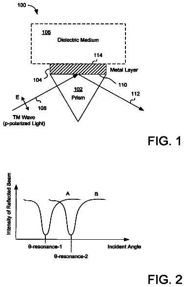
FIG. 1 is a flow chart of a method for determining the surface relaxivity of a medium.
FIG. 2 is a diagram of an NMR pulse diagram sequence used for determining the surface relaxivity of a medium.
FIGS. 3 a -3 e are DT.sub.2 distribution plots and fitting results for five different diffusion encoding times for a medium with elements having a first diameter size.
FIG. 3 f is a T.sub.2 distribution for the medium having a first diameter size.
FIGS. 4 a -4 e are DT.sub.2 distribution plots and fitting results for five different diffusion encoding times for a medium with elements having a second diameter size.
FIG. 4 f is a T.sub.2 distribution for the medium having a second diameter size.
FIGS. 5 a -5 e are DT.sub.2 distribution plots and fitting results for five different diffusion encoding times for a Berea sandstone rock core sample.
FIG. 5 f is a T.sub.2 distribution for the Berea sandstone rock core sample.
FIGS. 6 a -6 e are DT.sub.2 distribution plots and fitting results for five different diffusion encoding times for a Fontaineblue sandstone rock core sample.
FIG. 6 f is a T.sub.2 distribution for the Fountainblue sandstone rock core sample.
FIG. 7A shows a wireline NMR instrument deployed in a wellbore.
FIG. 7B shows a logging while drilling NMR instrument deployed in a wellbore.
Before turning to the drawings, an understanding is useful of some of the physics underlying hereinafter-described embodiments.
The time dependent diffusion coefficient in porous media depends on surface volume ratio S/V. See, e.g., Mitra, P. P. et al., “Diffusion propagator as a probe of the structure of porous media,” Physical Review Letters, Vol. 68, pp. 3555-3558 (1992); and Mitra, P. P. et al., “Short-time behavior of the diffusion coefficient as a geometrical probe of porous media,” Physical Review B, Vol. 47, p. 8565 (1993). In the short time limit, i.e. where the characteristic diffusion length (√{square root over (2D.sub.0Δ)}) is much smaller than the pore size, the apparent diffusion coefficient decrease is proportional to S/V, described by
D ( Δ ) D 0 = 1 - 4 9 π S V D 0 Δ , ( 1 ) where D.sub.0 is the bulk diffusion coefficient and Δ is the diffusion time. In the long time limit, D(Δ) approaches the asymptotic value D(∞)/D.sub.0=α. A Padé approximation can be used to connect the two limits,
D ( Δ ) D 0 = 1 - ( 1 - α ) β L D ( S V ) + ( 1 - α ) ( L D L M ) 2 ( 1 - α ) + β L D ( S V ) + ( 1 - α ) ( L D L M ) 2 ( 2 ) Where
β = 4 9 π , L D = D 0 Δ , and L.sub.M is the length scale characterizing the transition between the short-time and long-time diffusion limit. See, Latour, L. L., et al., “Time-dependent diffusion coefficient of fluids in porous media as a probe of surface-to-volume ratio,” Journal of Magnetic Resonance, Series A, Vol. 101 pp. 342-346 (1993); and Hürlimann, M., et al., “Diffusion-relaxation distribution functions of sedimentary rocks in different saturation states,” Magnetic Resonance Imaging, Vol. 21, pp. 305-310 (2003).
NMR T.sub.2 relaxation time is also affected in porous media by the surface to volume ratio as described by the expression
1 T 2 s = ρ S V ( 3 ) where T.sub.2s is the transverse relaxation time due to surface relaxation (where
1 T 2 s = 1 T 2 - 1 T 2 b , with T.sub.2b being the bulk relaxation) and ρ is the surface relaxivity. Combining equations
and
leads to a formula relating T.sub.2s and D(Δ):
D ( Δ ) D 0 = 1 - ( 1 - α ) β L D ρ T 2 s + ( 1 - α ) ( L D L M ) 2 ( 1 - α ) + β L D ρ T 2 s + ( 1 - α ) ( L D L M ) 2 ( 4 ) It should be appreciated that the use of a single transition length L.sub.M in equation
causes equation
to be effective for uniform pore size samples but does not necessarily address the case of a wide pore size distribution such as in rock formations. It should also be appreciated that in cases involving very large pores and low surface relaxivity where T.sub.2s approaches infinity, equation
reduces to
0 D ( Δ ) D 0 = 1 + α ( L D L M ) 2 1 + ( L D L M ) 2 . ( 5 ) As 0<α<1 and
L D L M is finite using a fixed L.sub.M, equation
does not asymptote to the bulk diffusion coefficient.
In order to permit equation
to be effective for a wide pore size distribution and have it approach the bulk diffusion coefficient when T.sub.2s approaches infinity, a parameter Γ is introduced such that L.sub.M is defined by
L M = Γ * V S = Γ ρ T 2 s ( 6 ) This definition causes L.sub.M to scale with pore size. For large pores, longer diffusion length is required to observe the transition between short-time and long-time diffusion limits. After introducing the new parameter, equation
will give the expected bulk diffusion coefficient in very large pores because as T.sub.2s approaches ∞, L.sub.M also approaches infinity. Substituting
into
now gives the mathematical description of the diffusion coefficient as a function of both diffusion encoding time Δ and relaxation time T.sub.2s with the desired asymptotic behaviors:
D ( Δ , T 2 s ) D 0 = 1 - ( 1 - α ) β L D ρ T 2 s + ( 1 - α ) ( L D Γ ρ T 2 s ) 2 ( 1 - α ) + β L D ρ T 2 s + ( 1 - α ) ( L D Γ ρ T 2 s ) 2 . ( 7 )
In one aspect, the generalized model in equation
can now be applied to samples with a wide distribution of pore sizes. Each pore size has a distinct diffusion coefficient D(Δ) and T.sub.2s, governed by equations
and
respectively. For a fixed value of T.sub.2s, equation (7), as a function of diffusion time Δ, reduces to the conventional Padé approximation of time dependent diffusion coefficient whose fitting yields the local surface to volume ratio S/V that is relevant to the NMR measurements. For a specified diffusion time Δ, equation
is a function of T.sub.2s. In the special case where T.sub.2s approaches ∞, i.e. very large pores, equation
reduces to
D ( Δ , T 2 s ) D 0 = 1 - 4 9 π 1 ρ T 2 s D 0 Δ ( 8 ) which is consistent with the known short-time limit models. See, Zielinski, L., et al., “Restricted Diffusion Effects in Staturation Estimates from 2D Diffusion-Relaxation NMR Maps,” SPE Annual Technical Conference and Exhibition (2010).
Turning now to FIG. 1 , an embodiment of a method for determining surface relaxivity of a porous medium is provided. At 10 , an NMR tool such as may be used in conjunction with a core analyzer uphole or such as a downhole tool described hereinafter with respect to FIG. 7A or 7B is activated to generate a pulsed field gradient NMR pulse sequence and data (decay signals over time τ) are collected. The pulse sequence is seen in FIG. 2 and may be utilized to obtain a DT.sub.2 distribution containing information about the geometry of a porous medium from which surface relaxivity information may be obtained as described hereinafter. The pulse sequence of FIG. 2 includes on a first channel, two spaced RF pulses of ninety degrees followed by a CPMG sequence of a ninety degree pulse followed by a series of one hundred eighty degree pulses, with signal acquisition prior to and between the one hundred eighty degree pulses, and on a second channel, a gradient pulse between the two spaced RF pulses of ninety degree pulses, a crusher pulse between the second RF pulse and the ninety degree pulse of the CPMG sequence, and another gradient pulse between the ninety degree pulse and the first echo of the CPMG sequence. The separation of the two gradient pulses is the diffusion encoding time Δ. As will be discussed hereinafter, according to one aspect, the pulse sequence of FIG. 2 is repeated for multiple different diffusion times, and for each diffusion encoding time, the pulse sequence is repeated for multiple different encoding strengths (q). In one embodiment, the encoding strengths increase in amplitude from pulse sequence to pulse sequence. In one embodiment, a first pulse sequence (q.sub.0) has gradient pulses having a strength of zero; i.e., they are not present. It will be appreciated that any of many techniques may be used to encode for D(Δ) each with its own advantages and disadvantages with respect to performance and sensitivity to artifacts. See, e.g., Price, W. S., “Pulsed-field gradient nuclear magnetic resonance as a tool for studying translation diffusion: Part 1. Basic theory,” Concepts in Magnetic Resonance, 9(5), pp. 299-336 (1997). Furthermore the pulse sequence components encoding for diffusion and T2 need not be in separate sections in time but may be combined together to simultaneously encode for both. For example, the ordinary CPMG sequence can be made to correlate diffusion and relaxation (T2) in a permanent gradient by, instead of varying a gradient strength, varying the echo time (te) of the entire CPMG. In this way the signal decay rate incorporate both diffusion and T2 information and varying te changes the sensitivity to diffusion and the effective diffusion encoding time (Δ) is the echo time (te). Accordingly, it should be understood that diffusion editing in the context of the present application may encompass (a) diffusion encoding that is a separate sequence from the T2 encoding sequence and (b) diffusion encoding that is at least partially integrated into the T2 encoding sequence.
Returning to FIG. 1 , at 20 , a DT.sub.2 distribution is determined from the NMR tool signals M(q, τ) resulting from the pulse sequences of different gradient strengths. More particularly, under Gaussian approximation the measured signal by pulsed gradient stimulated echo (PGSTE) followed by CPMG detection is described by
M ( q , τ ) = ∫ ∫ f ( T 2 , D ) ⅇ - γ 2 g 2 δ 2 D Δ ⅇ - τ T 2 ⅆ D ⅆ T 2 ( 9 ) where f(T.sub.2,D) is the DT.sub.2 distribution, γ is proton gyromagnetic ratio, g is pulsed gradient strength, δ is gradient duration, D is the apparent diffusion coefficient (which includes the effect of restricted diffusion), Δ is diffusion encoding time (of the gradient pulse sequence) and τ is the time in CPMG decay. The encoding strength is characterized by q=γgδ. As previously mentioned, for a given diffusion encoding time, the encoding strength is varied for a series of pulse sequences. This is accomplished by changing the pulsed gradient strength g, and/or by changing the gradient duration δ while keeping Δ fixed. Thus, M(q,τ) are the measured values for discrete values of q and τ and the collected data may be expressed as M(q.sub.i,τ.sub.j).
In some implementations, a 2D fast Laplace inversion algorithm is used to obtain the DT.sub.2 distribution f(T.sub.2, D) (for a particular diffusion encoding time Δ) from the measured values M(q,τ). See, e.g., Venkataraman, L., et al., “Solving Fredhom integrals of the first kind with tensor product structure in 2 and 2.5 dimensions,” Signal Processing, IEEE Transactions Vol. 50 pp. 1017-1026 (2002); and Song, Y.-Q., et al., “T1-T2 Correlation Spectra Obtained Using a Fast Two-Dimensional Laplace Inversion,” Journal of Magnetic Resonance, Vol. 154 pp. 261-268 (2002). More particularly, equation
may be rewritten as
M ( q i , τ j ) = Σ k , l f ( T 2 , k , D l ) ⅇ - q i 2 D l Δ ⅇ - τ i T 2 , k ( 9 a ) which represents a linear system of equations that can be solved using a fast numerical Laplace inversion (FLI). The result is a distribution or map of signals as a function indexed by their value of T.sub.2 and D; f.sub.T.sub. 2,k .sub.,D.sub. l .
From the DT.sub.2 distribution (also called a “DT.sub.2 map”), according to some implementations, a mean or average diffusion coefficient for a particular Δ is calculated by
D _ ( Δ , T 2 s ) = Σ i f ( T 2 s , D i ) * D i 2 Σ i f ( T 2 s , D i ) * D i ( 10 ) which results in a diffusion coefficient as function of both T.sub.2s and diffusion encoding time Δ. More particularly, and as seen in FIG. 1 at 30 , T.sub.2 indices are converted into T.sub.2s indices for the DT.sub.2 distribution data matrix f.sub.T.sub. 2,k .sub.,D.sub. l by relabeling the T.sub.2 index (data axis) as a T.sub.2s index (data axis) utilizing
1 T 2 s = 1 T 2 - 1 T 2 b . Then, at 35 , the average diffusion coefficient D is found as a function of T.sub.2 according to equation (10). Because magnetization signal decay is usually slowed down at large wave vectors due to the non-Gaussian behavior of restricted diffusion which potentially yields a secondary slow diffusion artifact peak, the D (Δ,T.sub.2s) calculation of equation
weights more strongly the large diffusion coefficients. As a result, the effect of non-Gaussian behavior is minimized to give a more accurate determination of the apparent diffusion coefficient. In another embodiment, instead of utilizing equation (10), the average diffusion coefficient is calculated according to
D _ ( Δ , T 2 s ) = Σ i f ( T 2 s , D i ) * D i 2 Σ i f ( T 2 s , D i ) . ( 10 a ) In some implementations, instead of utilizing equation
or equation (10a), the average diffusion coefficient is calculated according to
0 D _ ( Δ , T 2 s ) = Σ i f ( T 2 s , D i ) * D i Σ i f ( T 2 s , D i ) . ( 10 b )
At 40 , the T.sub.2 distribution across diffusion coefficients D.sub.i for a particular diffusion time Δ is calculated according to g (Δ, T .sub.2s)=Σ.sub.D.sub. i f .sub.Δ( T .sub.2s ,D .sub.i)
Then, at 50 , a determination is made as to whether data for all diffusion times Δ have been obtained and/or processed. If not, the method is repeated for a new diffusion time by generating a pulsed field gradient NMR pulse sequence with the new diffusion time and collecting data at 10 , determining the DT.sub.2 distribution at 20 , finding the average diffusion coefficient D at 35 (after relabeling at 30 ), and calculating the T.sub.2 distribution across diffusion coefficients D.sub.i at 40 . It is noted that instead of sequentially generating the pulse sequence and collecting data followed by determining the DT.sub.2 distribution, finding the average diffusion coefficient, etc., some or all pulse sequences may be generated and data collected prior to determining the DT.sub.2 distribution, finding the average diffusion coefficient, etc.
With the T.sub.2 distributions and the average diffusion coefficients D calculated for all Δ, it is then possible to make a determination of the surface relaxivity ρ. More particularly, at 60 , a minimization procedure is utilized where equation
is fitted to the 2D data set D (Δ,T.sub.2s) in order to extract a determination of the surface relaxivity ρ along with other (unknown) parameters such as the bulk diffusion coefficient D.sub.0, the asymptotic value α=D(∞)/D.sub.0, and parameter Γ=L.sub.m/ρT.sub.2s. In the minimization procedure, the cost function is constructed as follows: err=Σ.sub.Δ,T.sub. 2s {g (Δ, T .sub.2s)*[log D .sub.fit(Δ, T .sub.2s)−log D (Δ, T .sub.2s)]}.sup.2
where D.sub.fit(Δ,T.sub.2s) is the fitted function of equation
whose unknown parameters are chosen to cause the fitted function to most nearly approximate the data set of average diffusion coefficients, thereby causing equation
to be a minimum, and g(Δ,T.sub.2s) is the error weighing function, i.e. the T.sub.2 distribution calculated according to equation (11). In the minimization of equation (12), a logarithmic error is used so that it equally weighs the faster and slower diffusion coefficients (due to different pore sizes). In other embodiments, equation
is modified to include a non-logarithmic error. In those other embodiments, the slower diffusion coefficient region will have little effect on the fitting.
Alternatively or additionally, in order to generate a function relating Diffusion and T2, from a DT2 map, one can also calculate various weighted means T.sub.2s as a function of diffusion (e.g., T.sub.2s (D.sub.Δ)) to compute the functional relation between D and T.sub.2. For example, the log mean T.sub.2 as a function of D:
T 2 s _ ( D Δ ) = 10 Σ i F ( T 2 s , i , D Δ ) log 10 T 2 s , i Σ i F ( T 2 s , i , D Δ ) or the linear mean
T 2 s _ ( D Δ ) = Σ i F ( T 2 s , i , D Δ ) T 2 s , i Σ i F ( T 2 s , i , D Δ )
In some implementations, the pulsing at 10 , the determining of the DT.sub.2 distribution at 20 , the relabeling at 30 , the finding of the average diffusion coefficient D as a function of T.sub.2 according to equation
at 35 , and the calculation of a T.sub.2 distribution at 40 are done for a single encoding time Δ, and equation
is fitted to D (T.sub.2s) in order to extract a determination of the surface relaxivity ρ along with other (unknown) parameters such as the bulk diffusion coefficient D.sub.0, the asymptotic value α=D(∞)/D.sub.0, and parameter Γ=L.sub.m/ρT.sub.2s.
According to one aspect, it will be appreciated that the method of FIG. 1 is accomplished utilizing information obtained from NMR data only, and does not require other non-NMR measurements such as measurements of formation parameters such as porosity.
According to one embodiment, multiple determinations of surface relaxivity may be made along a distance or depth in a borehole and the determinations may be displayed as a log according to distance or depth in a borehole. According to another embodiment, the determination of surface relaxivity may be displayed on paper or on a screen.
In order to confirm the method of FIG. 1 , four packed glass beads (class IV soda lime spheres) were used as a model system. The glass beads had nominal diameters of 50 μm, 100 μm, 200 μm and 500 μm respectively. The diameter variation was about ±15% and spherical percentage was greater than 85%. The as-received glass beads were cleaned with 1M HCl at room temperature for one hour and then thoroughly washed with deionized water to remove paramagnetic impurities and surface contaminations. The cleaned glass beads were saturated with deionized water whose bulk relaxation time T.sub.2b was 2.3 s. The beads' pack information with respect to bead sizes, porosities and T.sub.2 relaxation times are summarized in Table 1 below.
In accordance with FIG. 1 , NMR measurements were carried out on a Magritek Rock Core Analyzer (.sup.1H frequency 2 MHz) at room temperature. The gradient was calibrated using bulk deionized water in 3 mm capillaries to avoid convection. Pulsed gradient stimulated echo (PGSTE) was used for diffusion encoding and the standard CPMG was used for data acquisition as depicted in FIG. 2 . The echo time TE between two π pulses was 167 μs. Signal decay due to diffusion in background gradient (<0.02 G/cm) during the CPMG acquisition was negligible.
The measured signal resulting from the NMR pulse sequences was processed according to FIG. 1 . Representative fitting results on glass beads are shown in subplot FIGS. 3 a -3 e (100 μm beads) and FIGS. 4 a -4 e (500 μm beads). The D (Δ,T.sub.2s) data are displayed in gray scale according to the weighing function g(Δ,T.sub.2s), i.e. T.sub.2 distribution. On each subplot, g(Δ,T.sub.2s) has been normalized for display purposes. Restricted diffusion is clearly seen as diffusion time increases from 40 ms ( FIGS. 3 a and 4 a ) to 1 s ( FIGS. 3 e and 4 e ), but the T.sub.2 distribution as seen in FIGS. 3 f and 4 f remains similar for all DT.sub.2 maps except the intensity decreases. Equation
is able to fit the diffusion coefficient behavior depending on T.sub.2 relaxation time and diffusion coefficient very well.
The multiple DT.sub.2 global fitting parameters are summarized in Table 1. Bulk liquid diffusion coefficient D.sub.0 varies a little bit because temperature is not strictly controlled and the water diffusion coefficient depends sensitively on temperature. The resultant long time limit diffusion coefficient D(∞)/D.sub.0α falls between 0.59 to 0.66, close to the expected value α=√{square root over (φ)}=0.62 for packed glass beads with porosity φ of about 0.37. It is interesting to note that the parameter Γ stays fairly constant although the bead diameter changed from 50 μm to 500 μm. This result is in agreement with the above suggestion that L.sub.M scales with pore size (and bead size).
TABLE-US-00001 TABLE 1 Sample information and multiple DT.sub.2 global fitting results based on eq. (7). size range porosity D.sub.0 Sample name (μm) φ T.sub.2 (s) ρ (μm/s) (10.sup.−9 m/s.sup.2) α Γ 50 μm bead 45-63 37% 0.27 14.9 2.19 0.66 2.5 100 μm bead 90-125 36% 0.48 16.5 2.18 0.62 2.1 200 μm bead 180-250 37% 0.66 21.8 2.15 0.62 2.1 500 μm bead 425-600 38% 1.19 20.7 2.22 0.59 1.9 Berea Null 23% distribution 19.4 2.15 0.56 2.1 Fontainebleau Null 5.6% distribution 3.0 2.15 0.62 1.9
To further estimate the reliability of the method, the fitted surface relaxivity ρ was compared to the value calculated by
ρ = d * ϕ 6 * T 2 s * ( 1 - ϕ ) ( 13 ) where φ is porosity and d is nominal bead size. Here
6 * ( 1 - ϕ ) d * ϕ can be used as a good estimate of surface volume ratio S/V because the bead size is fairly uniform and bead shape is mostly spherical. Since the diffusion length is in the order of micrometers, the surface roughness in nanometer scale should not affect the NMR relevant S/V. The calculated surface relaxivity using the method of FIG. 1 are shown in Table 2 along with single DT.sub.2 fitting results using fixed L.sub.M=100 μm and L.sub.M=20 μm respectively.
TABLE-US-00002 TABLE 2 Comparison between multiple DT.sub.2 global fit and fixed L.sub.M single DT.sub.2 fit Single DT.sub.2 Single DT.sub.2 Nominal Calculated L.sub.M = 100 μm, L.sub.M = 20 μm, bead size ρ (μm/s) Multiple DT.sub.2 Δ = 82 ms, Δ = 82 ms, d by Eq. 13 ρ (μm/s) ρ (μm/s) ρ (μm/s) 50 μm 16.0 14.9 10.1 12.2 100 μm 15.5 16.5 9.8 13.9 200 μm 21.2 21.8 12.6 28.2 500 μm 20.7 20.7 17.1 Null It is interesting to note that multiple DT.sub.2 fitted surface relaxivity is consistent with the calculated value for all four beads within a ±7% error. However, fixed L.sub.M parameterization on a single DT.sub.2 fitting, while providing a fairly good estimate for a specific bead size, is seen to not satisfy all pore sizes with multiple length scales. For example, while the fitting on 500 μm beads using L.sub.M=100 μm yields ρ=17.1 μm/s, which is only 17% smaller than the calculated 20.7 μm/s using equation (13), on 100 μm beads, it yields ρ=9.8 μm/s which is 37% smaller than the expected surface relaxivity 15.5 μm/s. The misfit is even more serious for a smaller fixed L.sub.M, for instance, L.sub.M=20 μm. For L.sub.M=20 μm, the 500 μm beads could not be fitted with this parameterization because the asymptotic value in equation
is significantly below 1.
NMR DT.sub.2 experiments were also carried out on Berea sandstone sample (porosity 23.17%, permeability 1026 mD) and Fontainebleau sandstone sample (porosity 5.63%, permeability 5.15 mD) rock cores where the multiple DT.sub.2 global fitting method of FIG. 1 was applied to determine the surface relaxivities of the samples. FIGS. 5 a -5 e show the results on the Berea sandstone rock core sample with a wide T.sub.2 distribution indicated in the subplot of FIG. 5 f . As diffusion time increases, the smaller T.sub.2 components gradually disappear, shifting the T.sub.2 distribution peak towards larger T.sub.2 values. The fitting of the method yields a surface relaxivity 19.3 μm/s, which is almost twice that of a previously reported value (9.8 μm/s) on a Berea sample with porosity 22% and permeability 380 mD. However, the previously reported value was based on a T.sub.2 distribution peak of 1.0 s while the measured T.sub.2 peak of this experiment was at 0.60 s. Thus, the difference in surface relaxivity might be caused by lithology or pore size differences. In FIGS. 5 a -5 e , it can be seen that the global fitting based on equation
works very well for smaller diffusion time, but an apparent deviation is observed for Δ=500 ms where the D (Δ,T.sub.2s) data lie below the fitted curve for the small and large T.sub.2 region. The D (Δ,T.sub.2s) data has a saddle-like shape, probably due to an internal gradient and the resolution limit of the fast Laplace inversion algorithm on a weak signal. However, this is accounted for by the weighing of the T.sub.2 distribution which focuses more on the well-behaved region. With the method of FIG. 1 , the effect of an abnormally small T.sub.2 and a large T.sub.2 region is minimal because the corresponding signal is very weak.
Fontainebleau sandstone results are shown in FIGS. 6 a -6 e . The T.sub.2 distribution shown in FIG. 6 e is between 1 s and 2 s, indicating a relative narrow pore size distribution. However some abnormal features are present on the D (Δ,T.sub.2s) data. For example, on the Δ=40 ms data, the diffusion coefficient decreases with T.sub.2 relaxation time. This could be caused by the resolution of the 2D inversion considering the narrow T.sub.2 distribution and the weak signal due to low porosity. The error due to 2D inversion can be averaged out to give a reasonable fitting result. The fitted surface relaxivity is 3.0 μm/s and other parameters fall into the expected range (Table 1). The small surface relaxivity is in line with the lithology and confirmed by the qualitative observation that its T.sub.2 peak is at 1.36 s, much larger than that of Berea sandstone (0.60 s), even though its pore sizes are smaller than that of Berea. Prior work reported surface relaxivities in the range 5-10 μm/s on a suite of 7 Fontainebleau sandstone samples. Particularly, on a Fontainebleau sample (porosity 6.4%, permeability 5.4 mD) similar to the investigated one, a surface relaxivity 5.1 μm/s was obtained. While the relaxivity determination obtained using the method of FIG. 1 of 3.0 μm/s is smaller than reported value of 5.1 μm/s, the results are consistent with the fact that the reported T.sub.2 distribution peak was at 0.83 s while the T.sub.2 distribution peak in the experiment was at 1.36 s.
It should be appreciated that the method of FIG. 1 may be carried out by any of numerous apparatus. Thus, in one embodiment, the method may be accomplished in an (uphole) laboratory through the use of a core sampler NMR apparatus such as, by way of example only, a Magritek Rock Core Analyzer. In another embodiment, the method may be accomplished utilizing downhole equipment such as shown in FIG. 7A or 7B .
FIG. 7A shows an example nuclear magnetic resonance (“NMR”) wireline well logging instrument 110 disposed in a wellbore 117 drilled through subsurface rock formations 126 , 124 . The instrument 110 is attached to one end of an armored electrical cable (“wireline”) 118 . The cable 118 may be extended into the wellbore 117 and withdrawn therefrom by a spooling device such as a winch 120 of types well known in the art. The cable 118 includes one or more insulated electrical conductors and may include one or more optical fibers to communicate signals between the instrument 110 and a recording unit 122 disposed at the Earth's surface. The recording unit 122 may include a processor or computer having an optional screen or printer type data display, input controls and a data recording device for storage of signals (e.g., NMR measurements) communicated from the well logging instrument 110 , as well as for storing or displaying calculated results made from NMR measurements made by the instrument 110 as described hereinafter. The well logging instrument 110 may also include a downhole processor as described hereinafter.
The NMR instrument 110 includes a magnet 112 for inducing a static magnetic field in the formations 124 , 126 having a predetermined spatial distribution of magnetic field amplitude. According to one aspect, magnet 112 may be supplemented by an electromagnet configured to impart a selected magnitude gradient field superimposed on the static homogenous field. The NMR instrument 110 may be arranged as disclosed in U.S. Patent Application Publication No. 20140184220, and/or in U.S. Pat. No. 5,796,252 which are both hereby incorporated by reference herein in their entireties. As the instrument 110 is moved along the interior of the wellbore 117 , nuclei in the formations surrounding the wellbore are magnetically polarized along the direction of the magnet's 112 field. The instrument 110 also includes an antenna for inducing radio frequency (“RF”) magnetic fields in the formations, and for detecting radio frequency signals induced by NMR phenomena excited in the formations by the static and RF magnetic fields. The particular portion of the formations adjacent to the wellbore from which the NMR signals originate depends on, among other factors, the spatial amplitude distribution of the static magnetic field and the RF frequency used to induce NMR phenomena in the formations. Some magnets may induce a region of substantially homogeneous field amplitude in a particular region in the formations; other types of magnets may induce static fields having a selected amplitude gradient in a particular region of interest. However arranged, the NMR instrument 110 is equipped to generate NMR pulses such as shown in FIG. 2 .
The description continues in the full USPTO document.
About 6,824 words. The USPTO PDF has it with every drawing.
Fees are due 3.5, 7.5 and 11.5 years after grant. This patent expired on November 21, 2025, so the fee marked "not paid" was the one that went unpaid.
METHODS AND SYSTEMS FOR DETERMINING SURFACE RELAXIVITY OF A MEDIUM USING NUCLEAR MAGNETIC RESONANCE
Filed Nov 2014 · published May 2016Methods and systems for determining surface relaxivity of a medium using nuclear magnetic resonance
Filed Nov 2014 · granted Nov 2017Earlier publications, parents and continuations. None of them can still be enforced, or this patent would not be listed.
Prior art cited by the examiner or applicant. Useful when you check your own idea for novelty.
Everything on this page comes from the documents linked above.