Automated method of identifying stock indexes which are historically high or low relative to a plurality of macroeconomic indicators

Background of the invention

Investors and their advisors have two basic tasks, namely, to find and buy low priced assets and then to sell those assets near their highest price. However, identifying whether a given price is truly high or low is a difficult task. Logic and economic theory tells us that we shouldn't compare any two historical prices without first accounting for the change in their relative values over time (e.g., adjusting for inflation). While there are many illustrations of the need to adjust for inflation, there are no simple, fast, and interactive ways of performing such a calculation. Furthermore, the marketplace is not solely a reflection of inflationary pressures, rather there are many other economic forces at work.

Summary of the invention

Preferred embodiments of the present invention tracks hundreds of macroeconomic indicators, calculating their change over time, and using them to adjust closing stock index prices so that the historical stock index closing levels reflect the change in those macroeconomic indicators, allowing for a more useful analysis. Through the “Index Finder” feature, the present invention sorts thorough tens of thousands of datasets to find the stock indexes that are at or near either the high or low point of their historical pattern and to discover whether or not that pattern is statistically significant. The Index Finder then displays its findings as Buy or Sell Signals for the stock indexes that passes its analysis.

Preferred embodiments of the present invention also allow for the independent investigation of other relationships through the “DataFall” effect which presents the historical price data in a more intuitive form of a “frequency distribution curve.” Another preferred embodiment carries out trading instructions to purchase or sell a portfolio of stock index-related financial products based upon its rankings.

The DataFall effect also has utility outside of the financial sector, performing its unique form of analysis on any large set of chronologically ordered data. While preferred embodiments of the present invention described herein assist in the analysis and purchase of financial products, other embodiments can be deployed in fields such as logistics, transportation, marketing, politics and pharmaceuticals.

Brief description of the drawings

The foregoing summary, as well as the following detailed description of preferred embodiments of the invention, will be better understood when read in conjunction with the appended drawings. For the purpose of illustrating the invention, there are shown in the drawings embodiments that are presently preferred. It should be understood, however, that the invention is not limited to the precise arrangements and instrumentalities shown.

In the drawings:

FIGS. 1A-7 , taken together, are flowcharts of the processes for implementing preferred embodiments of the present invention.

FIGS. 8A-8C and 9A-9B show user interface display screens for implementing preferred embodiments of the present invention.

FIGS. 10A-33 illustrate the calculations that are performed on each dataset in accordance with one preferred embodiment of the present invention.

FIG. 34 is a frequency distribution table for a sample dataset in accordance with one preferred embodiment of the present invention.

FIGS. 35A-35S illustrate an animated graphical display of the DataFall effect shown in FIGS. 4A-4B .

FIG. 36 illustrates the final output screen of the DataFall effect shown in FIGS. 35A-35S .

FIGS. 37-42 are prior art scatterplots which show how different patterns of data produce different degrees of correlation.

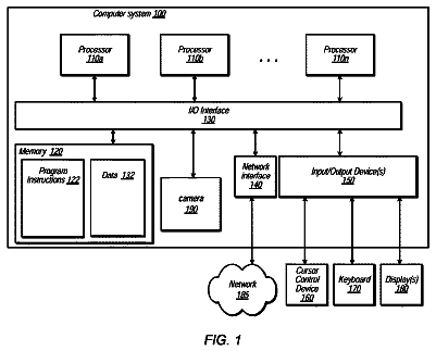
FIG. 43 is a hardware/software configuration in accordance with one preferred embodiment of the present invention.

Detailed description of the invention

Certain terminology is used in the following description for convenience only and is not limiting. Additionally, the words “a” and “an”, as used in the claims and in the corresponding portions of the specification, mean “at least one.”

The preferred invention will be described in detail with reference to the drawings. The figures and examples below are not meant to limit the scope of the present invention to a single embodiment, but other embodiments are possible by way of interchange of some or all of the described or illustrated elements. Moreover, where some of the elements of the present invention can be partially or fully implemented using known components, only portions of such known components that are necessary for an understanding of the present invention will be described, and a detailed description of other portions of such known components will be omitted so as not to obscure the invention. I.

Overview

FIGS. 1A-7 , taken together, are flowcharts of the processes for implementing preferred embodiments of the present invention. The flowcharts are also referred to herein as a Decision Tree Narrative. The flowcharts include steps 1-88 and are organized into three rows which represent the actions taken by the User (User), the user interface display (Display), and system processes (System).

Daily Data Update ( FIGS. 1A and 1B )

1. Start: Early every morning the system automatically begins the daily data update process. 2. Macro-Economic Indicator API: The system fetches specified macroeconomic data daily from the Federal Reserve of St. Louis's Economic Database (FRED) through the Application Program Interface. 3. Pro Rata Calculation: The system identifies the downloaded macroeconomic indicators as either daily, weekly, bi-weekly, monthly, quarterly or annual observations and transforms them into daily adjustment factors on a pro rata basis. The new daily adjustment factors are then added to the continuously updated Macroeconomic Database. 4. Stock Index API: System fetches the daily closing prices for specified stock indexes from publically available data sources. Save unadjusted daily closing price data on a Closing Price Database that is continuously updated with new price information. 5. Calculate Adjusted Stock Index Closing Prices: The system adjusts historical stock index closing prices by the appropriate daily macro-economic factors to create Realized Stock Index Prices. Save adjusted stock index closing price data on a temporary Realized Stock Index Database, which just lasts until the next set of datasets are calculated. 6. Calculate Lagged Adjusted Stock Index Closing Prices: The system then repeats the adjustment calculation from Step 5. on each stock index to account for a time lag between closing price and “proper” macroeconomic indicator of both a three-month and six-month delay. Save lagged, adjusted stock index closing price data on a Realized Stock Index Database, which lasts only until the next set of datasets are calculated. 7. Build Database of Dataset Frequency Distributions: Create a Frequency Distribution database table for each dataset (for each set of stock index, macroeconomic indicator & time lag variables) for the default time period (from Jan. 20, 1997 to the most recent closing price), which lasts only until the next set of datasets are calculated when a new most recent stock index closing price is calculated. 8. End: Databases are ready to perform Index Finder calculation and DataFall effect (as long as the default time period is selected). Index Finder ( FIGS. 2A-2C ) 9. Start: Data from prior section is calculated during the Daily Data Update and is available through the system to perform the calculations found in the Index Finder feature. 10. Single Dataset Analysis: each dataset (the Stock Index closing prices adjusted by macro-economic indicator and time lag) is first analyzed separately to check to see if it resembles a Bell Curve and if the most recent closing price is an outlier to its historical pattern. 11. Outlier Test: each dataset will be tested to see if the most recent closing price falls within a certain Administrator-defined percentage threshold which defines the highest and lowest data points in each dataset's historical price pattern. i. Fail: the dataset does not go on the Normal Distribution Curve Test, but skips to Step 24. ii. Pass: the dataset moves on to Step 12. 12. Positive/Negative Indicator: datasets with an outlier on the right-hand (Historically High) side of their frequency distribution curve will be assigned negative Shape Scores in Step 15. Outliers on the left-hand side (those that are on the Historically Low side of their price pattern), will be given positive Shape Scores in Step 15. 13. Normal Distribution Curve Test: each dataset that passes the Outlier Test will be submitted to a two-step test to see if the dataset's unique frequency distribution curve matches the idealized form of the Bell Curve, which is the basis for most standard forms of statistical analysis. a. Normal Probability Plot b. Test for Linearity In standard statistical models, the closer the dataset's frequency distribution curve comes to the ideal shape of the Bell Curve, the more credible that dataset is thought to be and the more predictive power it is believed to have. 14. Shape Score Assessment: the result of the Confidence Interval step of the Normal Distribution Curve Test will be given as a number between 0.00 & 1.00. The closer that number is to 0.00, the dataset will be revealed as randomly distributed. The closer that number is to 1.00, the dataset is said to be normally distributed. This number is the dataset's Shape Score. i. Fail: if the Shape Score is below an Administrator-defined threshold (e.g.: 0.5 or greater), the dataset is thought to be too randomly distributed to be credibly predictive, so it does not complete the Index Finder feature (skipping directly to Step 24). ii. Pass: the dataset moves on to Step 15. and becomes known as a “Qualified Dataset” 15. Positive/Negative Shape Score Assignment: the Shape Score of the dataset will become positive or negative based on where the Outlier sat on the Curve as determined in Step 12. 16. Stock Index Sorter: each Qualified Dataset are sorted according to which Stock Index it represents. Then each Stock Index's Qualified Dataset's Shape Score are added together to form a Combined Shape Score for each Stock Index. The system then ranks each Stock Index according to which Stock Index has the highest Combined Shape Score (in both the positive and negative directions). 17. Historically High/Historically Low: the highest negative Combined Shape Scores will be displayed under the “Historically High” listing in the Index Finder, which Users should interpret as a Sell Signal. The highest positive Combined Shape Score will be displayed as “Historically Low” in the Index Finder section of the website, which Users should interpret as a Buy Signal. The higher the Combined Shape Score (whether it is positive or negative), the stronger the signal to either Buy or Sell. 18. Frequency Distribution Table: all datasets, whether or not they passed the Outlier and/or Normal Distribution Curve Tests, are made available for the User to analyze in the User-Defined Dataset Analysis process. 19. User Opens Program: This is the first step that requires human intervention, Steps 1 to 18 in this process have been performed automatically by the system. This step opens the Selection Screen. 20. Selects a Stock Index from Index Finder: If the User chooses one of the Stock Indexes suggested to them by the Index Finder feature of the website, whether it is Historically High or Historically Low, move onto Step 21. If they do not chose a Stock Index through the Index Finder, move onto Step 24. 21. Dataset Selection Screen: the system displays a new screen, the Dataset Selection Screen, which presents to the User the datasets within the chosen Stock Index that have the highest Shape Score. Each dataset that is presented on this screen is clickable. 22. Selects Dataset to Analyze: if the User selects one of the suggested datasets to investigate further, they move on to step 30. If the User decides to close the Dataset Selection Screen without selecting a dataset, they will return to Step 20 (where they are able to choose either to select a new dataset or, later in the process, to create their own dataset). 23. Continue to Step 30: if the User selects a dataset from among those suggested on the Dataset Selection Screen, then the system fills in each of the Drop-Down boxes (Stock Index, Macro-Economic Indicator, and Time Lag) according the parameters of the selected suggested dataset, and the process moves ahead to Step 30. 24. End: if the User does not select a Stock from the Index Finder feature of the website, this phase of the program ends and all the Frequency Distribution Tables for the default time period (from Jan. 20, 1997 to the most recent market close) are made available to the User to analyze. These Frequency Distribution Tables only last until the next set of datasets is compiled when the next daily data update is performed. User-Defined Dataset Analysis ( FIGS. 3A-3D ) 25. Start: if the User does not use the Index Finder feature of the website, they can explore any dataset that they want to investigate through choices presented to them on the Selection Screen. 26. Selects/Changes Stock Index: the User selects a (or changes a previously selected) Stock Index to analyze from a drop-down box that provides a list of Stock Indexes that the system tracks. The drop-down list includes the names of the most popular Stock Indexes, plus an option for “More . . . ”. If the User selects one of the named Stock Indexes on the drop-down list, then slip Step 27 and move directly onto Step 28. 27. Stock Index Selection Screen: if the User selects the “More . . . ” option on the drop-down list, it opens a new screen, the Stock Index Selection Screen, that provides information about each of the Stock Indexes that the system tracks (including those already listed by name on the drop-down list), including: name, description, style (broad index, industry sector, capitalization size, or stock style), and price chart. Once the User clicks on the “Select” button, the Stock Index Selection Screen closes and they return to the Selection Screen with the name of the selected Stock Index in the drop-down box. 28. Index Inception Date Look-Up: the system automatically looks up the inception date (the date that the Stock Index was first tracked) for the Stock Index that was selected by the User. The oldest date available on the Closing Price Database is Aug. 15, 1971 (the day that the U.S. left the Gold Standard and the value of the U.S. Dollar began to be set mostly by market/economic conditions rather than government policy). If the inception date of the Stock Index was sometime after Aug. 15, 1971, then the oldest recorded closing price will become the inception date for that Stock Index. The Inception Date will be that Stock Index's oldest possible Start Date for determining the Time Period to be analyzed. 29. Historical Closing Price Data Look-Up: the system automatically looks-up the price history for the selected Stock Index from the earliest date to the most recent closing price. 30. Price Chart displays actual Closing Prices: the system displays the actual, unadjusted daily closing prices of the selected Stock Index from the earliest/oldest date available to the most recent closing price. This data is presented as a Red Line on the Price Chart. The y-axis of the Price Chart is the price values and the x-axis are the dates for each observation. The x-axis and y-axis are scaled so that the chart only displays values that are represented in the data. The Time Slide (under the Price Chart) reflects the time period being displayed. The Time Slide runs from the Stock Index's Inception Date (with a maximum date of Aug. 15, 1971) to the most recent market close. The Start Date of the Time Period defaults to Jan. 20, 1971 (when the NASDAQ implemented new Small Order Execution System, “SOES”, rules, which along with other contemporaneous rules changes, fundamentally altered the nature of the stock market), but the Start Date can be changed by the User. The End Date cannot be changed by the User, it is always the most recent market close. 31. Did the User adjust the time period?: the Index Finder feature only looks at data for closing prices between Jan. 20, 1997 and the most recent market close. However, in the User-Defined Dataset Analysis section, the User can change the time period being examined by changing the Start Date on the Time Slide. The User can select a Start Date from Aug. 15, 1971, but it defaults to Jan. 20, 1997. The End Date will always be the most recent market close. If the User changed the time period, move on to Step 32. If they did not, skip to Step 33. 32. Update Price Chart: a change in the Start Date will be reflected in a new x-axis scale and Time Slide, as well as a change in the Red Line to reflect the new time period. 33. Select/Change Macroeconomic Indicator: the User next selects a (or changes a previously selected) Macroeconomic Indicator upon which to base the analysis from a drop-down box that provides a list of Macroeconomic Indicators that the system tracks. The drop-down box is populated with a list of ten most often used Macroeconomic Indicators, along with an option for “More . . . ”. If the User selects one of the Macroeconomic Indicators named on the drop-down list, then slip Step 34 and move directly onto Step 35. 34. Macroeconomic Indicator Selection Screen: if the User selects the “More . . . ” option on the drop-down list, it opens a new screen that provides information about each of the Macroeconomic Indicators that the system tracks (including those already listed by name on the drop-down list), comprising: name, category, description, and a historical chart. The Macroeconomic Indicator Screen also allows the User to use Inflation-Adjusted (CPI or PPI) and/or Per Capita numbers for each Macroeconomic Indicator (if appropriate). Once the User clicks on the “Select” button, the Macroeconomic Indicator Selection Screen closes and they return to the Selection Screen with the name of the selected Macroeconomic Indicator populating the drop-down box. 35. Adjust Time Period for Macroeconomic Indicator?: the system automatically checks to ensure that the inception date of the selected Macroeconomic Indicator is older than or equal to the date range selected by the User for the Stock Index. If “yes”, then return to Step 32. If “no”, move on to Step 36. 36. Adjusted Stock Index Prices Calculation: the system automatically calculates the Adjusted Stock Index Closing Prices (assuming a Time Lag of “None”). For each daily closing price, the system finds the change (increase or decrease) in the concurrent Macroeconomic Indicator on the Macroeconomic Database by dividing that day's level by the current level to produce an adjustment factor. The closing price for that day is then multiplied by that day's adjustment factor, which brings the old price “up to” today's price level. This process is repeated for each daily closing price in the selected time period. 37. Price Chart Updated with Adjusted Stock Index Prices: the system displays the Adjusted Closing Prices as a Yellow Line on the same Price Chart along with the Red Line that reflects the Actual Closing Prices. The x-axis values, its scale, and the Time Slide do not change, but the y-values and its scale will change as necessary to accommodate the new range of Adjusted Closing Price data. 38. Did the User adjust the time period?: the User may choose to change the selected time period being examined. If they do change the time period, move to Step 39. If they do not change the selected time period, it moves onto Step 40. 39. Price Chart Updates to Reflect Selected Time Period: the system updates the Price Chart to reflect the revised Time Period. The Yellow Line, Red Line, x-axis, y-axis, and Time Slide are all adjusted based on the new Time Period. 40. Selects/Changes Time Lag: lastly, the User selects a Time Lag to adjust the analysis by; their choices are “None”, “Three Months”, or “Six Months”. The purpose of this variable is to allow Users to test the concept that the stock market is a “forward-looking” pricing mechanism by comparing a historical price not to that same day's macroeconomic measure, but rather to a measure from three or six months into the future (depending on the length of the time lag). 41. Recalculate Adjusted Stock Index Prices for Selected Time Lag: if the User selects “None”, then no recalculation needs to take place. If the User chooses “Three Months”, then the Closing Stock Index Price for a particular day will be adjusted by the macroeconomic daily factor for the day three months in the future. If the User selects “Six Months”, then the Closing Stock Index Price for a particular day will be adjusted by the macroeconomic daily factor for the day six months in the future. 42. Update Price Chart for Time Lag: the system revises the display of the Price Chart to account for the change in the Adjusted Closing Stock Index prices, updating the x-axis values and scale (if necessary). 43. Did the User adjust the time period?: the User may choose to change the selected time period being examined. If they do change the time period, move to Step 44. If they do not change the selected time period, it moves onto Step 45. 44. Price Chart Updates to Reflect Selected Time Period: the system updates the Price Chart to reflect the revised Time Period. The Yellow Line, Red Line, x-axis, y-axis, and Time Slide are all adjusted based on the new Time Period. 45. User Clicks the “Next” Button: once the User is satisfied with their choice of Stock Index, Macroeconomic Indicator, Time Lag, and Time Period, the User can click on the “Next” button to move onto the DataFall Screen. If they later want to change the Stock Index, Macroeconomic Indicator, or Time Lag for the dataset, the User will need to return to the selection Screen (Step 25). The User will be able to adjust the Time Period (if desired) from the DataFall Screen. 46. Open the DataFall Screen: the Selection Screen does not close, it remains open “under” the new DataFall Screen so that the User can click back on it to return to the Selection Screen. The DataFall Screen is prepopulated with the variables for the dataset selected on the Selection Screen. The only variable that the User is able to alter on the DataFall Screen is the Time Period, which they can change through the Time Slide feature. 47. Database Supplies Adjusted Price History: the DataFall effect is populated by the data calculated in the above steps that created the final dataset. The database presents the dataset for the DataFall Screen in chronological order. 48. DataFall builds a Frequency Distribution Curve: this process is explained in greater detail in Steps 50-59. Once the Curve is created, the User can alter the Time Period through the Time Slide or return to the Selection Screen to change any of the other variables to create a new dataset to be examined. 49. End: the DataFall Effect allows the User to see the development of the Frequency Distribution Curve for the given dataset as it either develops into a normal distribution curve (a Bell Curve) or doesn't. If the frequency distribution does not look like a Bell Curve, then the dataset is not normally distributed and it can be assumed that there is no credible statistical &/or predictive relationship between the selected variables. If the frequency distribution curve of the dataset does resemble a Bell Curve, then the variables are correlated and, likely, predictive (as long as there are no substantial changes to the structure of the marketplace; as happened, for instance, on Jan. 20, 1997 when NASDAQ changed the SOES rules). DataFall Effect ( FIGS. 4A-4B ) 50. Start: the DataFall effect is a new method of visualizing large amounts of chronologically ordered data. In this case, the data being analyzed/visualized is the adjusted historical prices of stock indexes, but this method of looking at Big Data is applicable in many settings and industries such as marketing (e.g., strength of brand data), logistics (e.g., package delivery time), polling (e.g., approval ratings of politicians), pharmaceutical testing (e.g., pharmaceutical trial data) and transportation (e.g., common carrier arrival/departure time data). Thus, the scope of this preferred embodiment includes using the DataFall effect to visualize chronologically ordered data in fields other than stock index research. 51. User Clicks the “Next” Button: as in Step 45, once the User is satisfied with their choice of Stock Index, Macroeconomic Indicator, Time Lag, and Time Period, the User can click on the “Next” button to move onto the DataFall Screen. 52. Open the DataFall Screen: as per Step 46, the Selection Screen does not close, it remains open “behind” the new DataFall Screen so that the User can click back on it to return to the Selection Screen. The DataFall Screen is pre-set to match the variables for the dataset selected on the Selection Screen. The only variable that the User is able to alter on the DataFall Screen is the Time Period, which can be adjusted through the Time Slide feature. 53. Database Supplies Adjusted Price History: as in Step 47, the DataFall effect is populated by the data calculated in the above steps that created the final dataset. The database presents the dataset for the DataFall Screen in chronological order. 54. Data point Animation: the oldest data point in the dataset appears on top of chart at its x-axis value and drops vertically towards the bottom of the display. If there already is a data point at the bottom of the chart at that x-axis value, the newer data point “lands” on the oldest one, accumulating into a column (the frequency distribution histogram). Each data point is like a snowflake falling from the sky to land on the ground, accumulating into a “snow drift” at the bottom of the display to form the frequency distribution curve for the dataset being analyzed. As the Curve is being built, the directionality and momentum of the stock market can be seen by the User in the movement of the data points as they fall to the bottom of the screen. 55. Is there a next data point?: as each data point appears, becomes animated, and “falls” towards the bottom of the chart, the process cycles through this step. If there is another data point in the set, then return to Step 54, and the cycle continues to “build” the frequency distribution curve. If this is the last data point in the set (if the data point represents the most recent closing price), move on to Step 56. The User is able to adjust the speed of the DataFall effect by way of the DataFall Speed Slide, even to the point of “shutting off” the DataFall effect so that the frequency distribution histogram for the dataset simply appears fully completed instead of being built up as the User watches. 56. Last data point in the dataset is displayed in a contrasting color: if the Time Indicator check-off box is unchecked, then all the earlier data points are displayed in yellow, while the most recent closing price is displayed in red. If the Time Indicator check-off box is selected/checked, then the earlier data points are colored according to their time quintile (discussed in Step 64), but the most recent closing price is displayed in red. The contrasting color allows the User see instantly where the most recent price lands onto and fits into the dataset's frequency distribution curve. 57. Calculates the dataset's Mean and 200-Day Moving Average: the system automatically calculates the displayed dataset's mean (the x-axis value which marks the spot where half of the observations are to its left and half are to its right) and its 200-day trend (the line which smooths out the volatile variations in the actual frequency distribution histogram of the dataset). 58. Display Mean Line and Curve Line: display the dataset's mean with a red Mean Line and use a black Curve Line to represent the dataset's 200-day moving average. 59. Did the User adjust the time period?: the User may choose to change the selected time period being examined. If they do change the time period, move to Step 60. If they do not change the selected time period, it moves onto Step 61. 60. Repeat the DataFall and adjust Time Slide: the data points do not need to be recalculated for a new time period, the system must only determine the new range for the dataset based on the selected time period. The system then repeats Steps 53 to 58 in order to present the User with an updated DataFall presentation. The Time Slide below the DataFall Chart is updated to reflect the revised time period. 61. End: the DataFall effect not only presents the dataset in terms of whether or not its frequency distribution curve is normally or randomly distributed (or somewhere in between), it also allows the User to instantly and intuitively see if the most recent closing price is an outlier. If the most recent closing price is on the right-hand side of a dataset's frequency distribution curve which is also normally distributed (looks like a Bell Curve), then it is on the high side of its credible and predictive historical price pattern. If the most recent closing price is on the left-hand side of a dataset's Bell Curve shaped frequency distribution curve, then it is on the low side of its credible and predictive historical price pattern. Regression Towards the Mean is a widely accepted statistical “law” that holds that if the current observation is an outlier, then future observations are more likely to move closer to the center of the Curve than further out towards either tail. Therefore, when the most recent close is on the left-hand tail of a strongly shaped Curve, it is signal to sell or short that index; and when it's on the right-hand side of a well-formed Bell Curve, then it is a signal to buy that index. The more datasets for an index that repeat the same outlier/Bell Curve pattern, the stronger the Buy or Sell signal for that particular Stock Index. Time Indicator Check Box ( FIG. 5 ) 62. Start: as weather radar uses color to indicate the intensity of precipitation, the system uses color to indicate the chronology of the data points. The selected time period is divided into quintiles, with each quintile comprising of 20% of the observations (the first quintile being the oldest 20% of observations, the next 20% being the next oldest, and so on). When/if the User changes the time period being examined, the system will recalculate the time quintiles. 63. If the User selects the “Time Indicator” check: this process does not begin until the User chooses to check the “Time Indicator” check-off box. Otherwise, skip this entire process. 64. Multi-color DataFall: each time period quintile is assigned a color (the pattern of which is repeated on the Time Slide, allowing the Time Slide to also act as an interpretive guide as to the meaning of the colors). Then each data point in the DataFall animation is given the proper color for their quintile. The data points retain their color as they form the frequency distribution histogram for the dataset, allowing the User to see the time-bound patterns within the overall pattern of the price history. If the colors are evenly dispersed around the Curve, then there is no pattern to be discerned. If the colors “clump” together, then Users can take this fact into consideration. 65. User unselects “Time Indicator”: if the User un-clicks the “Time Indicator” check-off box, then the data points and Time Slide revert to their normal two-color palette. 66. Returns to two-color DataFall: the data points and Time Slide revert to their usual color pattern with all the data points in the same color (yellow) except for the data point representing the most recent closing price, which is displayed in a contrasting color (red). 67. End: the purpose of the multi-colored DataFall is to allow the Users to see if/where certain time periods may have developed their own short-lived price patterns. With this knowledge, the User can change the Time Period in order to eliminate that sub-pattern from their analysis. For instance, if all the data points on one tail of the Curve are in one color (and, therefore, from a single time quintile), changing the Start Date will allow the User to remove those outliers from the dataset being examined. Curve Morphing ( FIGS. 6A-6B ) 68. Start: DataFall analysis is designed to be as simple as possible, with the main driver of variation in the dataset being the Macroeconomic Indicator because we want to focus in on one causal factor at a time. Curve Morphing allows the User to examine two Macroeconomic Indicators, thereby creating a simplified version of multivariate analysis. The inspiration for the visual effect is based upon the practice of “photo morphing”, where the images of two distinct faces are merged together to form a third face that is “half-way inbetween” the original two faces. 69. If the User selects “Curve Morphing”: this process does not begin until the User chooses to check the “Time Indicator” check-off box. Otherwise, skip this entire process. 70. Rename DataFall Screen: the DataFall Screen that is currently opened becomes Screen One. 71. Remove Data Points: the Frequency Distribution histogram (all the data points for the dataset) disappear from Screen One, leaving only the Curve Line, the Mean Line, and the contrasting Dot representing the most recent closing price. 72. New Selection Screen Opens: the system automatically opens a new Selection Screen to allow the User to select a new dataset to analyze. The only limitation is that the User must select the same Stock Index was used in Screen One. 73. User Repeats Dataset Selection and Analysis: the User follows Steps 20 through 61, with the proviso that they cannot use a different Stock Index as the basis for their analysis, nor can they change the Time Period. The User completes the DataFall analysis process as normal, with the same Stock Index and Time Period, but different Macroeconomic Indicator and/or Time Lag. 74. New DataFall Screen Renamed: the new DataFall Screen is renamed Screen Two. As in Step 78, the histogram disappears, leaving only the Curve Line, the Mean Line, and the contrasting Dot representing the most recent closing price. 75. Morphing Calculation: the System aligns the Mean Lines of each dataset, then for every x-axis value to the left and right of the Mean, the system calculates the point that is midway between the y-axis value for Screen One and Screen Two at that x-axis value, creating a new Curve Line that is the average of the original two. 76. Morphing Screen: in a new Screen, the Morphing Screen, the Curve Lines from Screen One & Screen Two are animated so that they can be seen moving towards each other and then combining together into the third Curve Line, which is the average of the first two Curve Lines. 77. System calculates the average Most Recent Closing Price: the system “counts” the number of x-axis values that the Most Recent Closing Price from Screen One lies away from its dataset's mean, then it does the same for Screen Two. The system then calculate the average number of x-axis values that the two Screen's Most Recent Closing Price lies away from the Mean, this is now the Morphed Current Price for the combined Curves. 78. Display Morphed Current Price: the Curve Line on the Morphing Screen is updated to display the Morphed Current Price as a red dot on the Line. 79. End: when the User closes the Morphing Screen, Screen Two closes as well. Trade Execution ( FIG. 7 ) 80. Start: through the Index Finder, DataFall analysis, and Curve Morphing features the User is able to find Stock Indexes that are at either the high or low end of their historical price pattern. Those Stock Indexes that are historically high will, in due time, regress back to the mean of their price pattern, so they ought to be sold or shorted. Those Stock Indexes that are historically low will, in due time, regress back to the mean of their price pattern, so they ought to be bought. Thereby allowing Users to follow the only rule of investing: “Buy low, sell high.” 81. User selects “Trade” button: once the User is satisfied that they have found stock indexes that are at or near either their historical high or low, the User can execute their trades based upon their analysis through the system. 82. Display Equivalent Financial Products List: stock indexes cannot be bought or sold directly, Users need to find Mutual Funds and/or ETFs based on the stock indexes that they selected. The Equivalent Financial Product List not only displays those mutual funds and ETFs that directly correspond to the selected stock indexes, but also those that are leveraged and/or inversely related. Users select a financial product by clicking on the name. 83. Link to Trading Platform: once the User selects a financial product in Step 82, the system connects to a Trading Platform as a separate window fed by the system's information. 84. Display Trading Platform: the system displays the Trading Platform pages to the User 85. Input buy/sell instructions: the User inputs their trading instructions into the Trading Platform 86. Execute Trade: the system executes the User's trading instructions through the Trading Platform. The Platform makes the trade through a marketplace and sends confirmations. 87. Display Trading Confirmation: the system displays the trade confirmation to the User. 88. End: if the time-honored rules of statistics hold true, then the Users should be able to maximize their long-term investment's profits. II.

Detailed disclosure

FIGS. 8A-8C and 9A-9B show user interface display screens for implementing preferred embodiments of the present invention.

Selection Screen Narrative

Selection Screen ( FIG. 8A ): When the User logs onto the system, the first screen that is displayed is the Selection Screen, which is comprised of the following components.

The description continues in the full USPTO document.