 Lapsed, fee not paid5 drawings
Software & Apps · US 11,244,588 B2
Controlling refreshes of pixels in display devices
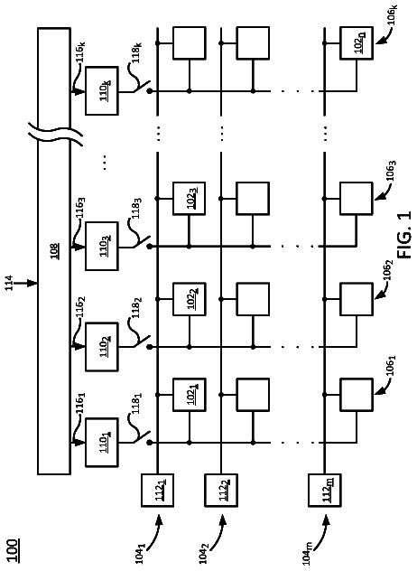
A display device includes pixels, a serial-to-parallel converter (SPC), a row driver, a column driver, and a switch.
US 11,245,593 B2 · Assignee: VMware, Inc. · Inventors: Knowles; Christopher et al.
Sheet 1 of 47 from the published document. All sheets in the USPTO PDF
The current document is directed to methods and systems for frequency-domain analysis of operational and performance metric values and other data generated and collected within computer systems, including large distributed computer systems and virtualized data centers. In one implementation, each set of time-ordered values for each metric in a set of metrics is partitioned into time intervals, transformed from the time domain to the frequency domain, and aligned to generate a metric surface in a frequency-time-amplitude space. The metric surfaces are then pairwise compared to identify related metrics. Transfer functions are generated for transforming metric surfaces into one another. The comparison values and transfer functions are used to produce graphs that encapsulate discovered relationships between metrics.
Initially, computers were large, monolithic, single-processor systems that sequentially executed programs, encoded on stacks of Hollerith cards, without the benefit of operating systems, communications networks, and programs compiled from modem computer languages. Over the past 60 years, computer systems have evolved to include a wide variety of system and device types, from hand-held smart phones and tablets, which provide computational bandwidths and data-storage capacities that are orders of magnitude greater than those provided by the initial computer systems of the mid-1950s, to vast, network-interconnected distributed computing systems that include thousands, tens of thousands, or more multi-processor servers, dedicated data-storage appliances, and communications networks. These distributed computing systems can each support multiple virtualized data centers, each comprising thousa
1 of 47 drawing sheets so far from the published document, cropped to the drawing. Every sheet is in the USPTO PDF.
What the patent claimed, word for word. All of it is now free to use.
The current document is directed to automated computer-system administration and management as well as automated tools to facilitate human administration and management of computer systems and, in particular, to methods and systems for frequency-domain analysis of time-ordered operational and performance metric values within computer systems.
Initially, computers were large, monolithic, single-processor systems that sequentially executed programs, encoded on stacks of Hollerith cards, without the benefit of operating systems, communications networks, and programs compiled from modem computer languages. Over the past 60 years, computer systems have evolved to include a wide variety of system and device types, from hand-held smart phones and tablets, which provide computational bandwidths and data-storage capacities that are orders of magnitude greater than those provided by the initial computer systems of the mid-1950s, to vast, network-interconnected distributed computing systems that include thousands, tens of thousands, or more multi-processor servers, dedicated data-storage appliances, and communications networks. These distributed computing systems can each support multiple virtualized data centers, each comprising thousands, tens of thousands, or more virtual servers interconnected with virtual networks to support execution of very large numbers of virtual machines that each, in turn, support execution of one or more applications.
While the operational state of an early, 1950s single-processor computer system could be represented by numerical values stored in a handful of status registers, the operational state of a large, modem, distributed computing system or virtualized data center may currently be obtained only by automated and semi-automated processing of megabytes, gigabytes, or terabytes of accumulated data to produce a large derived data set that represents the system state. Modern, distributed computing systems and virtualized data centers include many different types of components at a variety of different hierarchical levels of organization, each of which may be, in part, characterized by a variety of different numerical and textural status values and descriptions as well as collected sets of time-ordered operational and performance metric values. The performance, behaviors, operational characteristics, and corresponding metrics and state representations for the various components may vary over sub-millisecond time intervals, as in the case of processors, to seconds, as in the case of network components, to days and longer periods of time, as in the case of data-storage capacities. For certain components, such as collections of executing application programs and operating-system routines that are referred to as workloads, the state of, and operational and performance metrics associated with, workloads may exhibit time behaviors over a range of time intervals from milliseconds to days, weeks, and longer time intervals. Thus, not only are the data sets from which derived data sets that represent system operational states and performance are obtained voluminous, but they additionally involve time-dependent behaviors that vary over vastly differing characteristic time intervals.
As a result of the complexity of current distributed computer systems, including virtualized data centers, and the enormous amount of data that must be processed and analyzed in order to understand the performance and operational characteristics of the distributed computing systems so that the distributed computing systems can be rationally managed and administered, management and administration of modem computing systems is necessarily evolving from manual methods and processes to fully automated management and administration. Even with fully automated management and administration, the computational bandwidth, data-storage capacity, and communications-network bandwidth needed for automated management and administration of modern distributed computing systems may represent a significant fraction of the total bandwidth and capacity of the distributed computing systems. Designers, manufacturers, and vendors of distributed computing systems, as well as users and, ultimately, clients of distributed computing systems, therefore continue to seek new, efficient automated tools for processing and analysis of data generated within distributed computing systems, including operational and performance metric values, in order to implement automated management and administration components of distributed computing systems and to facilitate performance of remaining semi-automated administration and management tasks.
The current document is directed to methods and systems for frequency-domain analysis of operational and performance metric values and other data generated and collected within computer systems, including large distributed computer systems and virtualized data centers. In one implementation, each set of time-ordered values for each metric in a set of metrics is partitioned into time intervals, transformed from the time domain to the frequency domain, and aligned to generate a frequency-time-amplitude surface in a frequency-time-amplitude space. The frequency-time-amplitude surfaces are then pairwise compared to identify related metrics. In addition, in certain implementations, transfer functions are generated for transforming each of two surfaces corresponding to two metrics into the other of the two surfaces. The comparison values and transfer functions are used to produce graphs that encapsulate discovered relationships between metrics. These graphs can be used in automated administration and management systems for analysis of the operational and performance characteristics of the system, classification of system components, resource management and tuning, identification and diagnosis of problem states and anomalies, and for many other purposes.
FIGS. 1A-G illustrate the decomposition of a complex waveform into component sinusoids, a frequency-domain discrete spectrum of the complex waveform, and a mathematical context for describing complex waveforms as the sum of component sinusoids.
FIGS. 2A-B show expressions for Fourier transforms and illustrate the convolution operation.
FIG. 3 illustrates a simple Fourier pair.
FIG. 4 provides a general architectural diagram for various types of computers.
FIG. 5 illustrates an Internet-connected distributed computer system.
FIG. 6 illustrates cloud computing.
FIG. 7 illustrates generalized hardware and software components of a general-purpose computer system, such as a general-purpose computer system having an architecture similar to that shown in FIG. 4 .
FIGS. 8A-D illustrate two types of virtual machine and virtual-machine execution environments as well as containers.
FIG. 9 illustrates an OVF package.
FIG. 10 illustrates virtual data centers provided as an abstraction of underlying physical-data-center hardware components.
FIG. 11 illustrates virtual-machine components of a VI-management-server and physical servers of a physical data center above which a virtual-data-center interface is provided by the VI-management server.
FIG. 12 illustrates a cloud-director level of abstraction.
FIG. 13 illustrates virtual-cloud-connector nodes (“VCC nodes”) and a VCC server, components of a distributed system that provide multi-cloud aggregation and that include a cloud-connector server and cloud-connector nodes that cooperate to provide services that are distributed across multiple clouds.
FIGS. 14A-H illustrate metric-value data sets and generation of metric surfaces in frequency-time-amplitude space.
FIGS. 15A-F illustrate several types of operations that are carried out on metric surfaces.
FIGS. 16A-C illustrate two of many possible approaches to computing a relatedness value, or comparison metric, between two metric surfaces.
FIGS. 17A-B illustrate the overall comparison of two metric surfaces.
FIGS. 17C-D illustrate generation of a component graph based on frequency-time-amplitude-surface-comparison metrics and frequency-time-amplitude-surface transfer functions.
FIGS. 18A-B provide control-flow diagrams to illustrate one implementation of an automated metric-analysis subsystem within an automated administration and management subsystem of a distributed computing system.
FIG. 19 illustrates one approach to using frequency-domain data for classification.
The current document is directed to frequency-domain analysis methods and distributed-computing-system components that implement and facilitate automated and semi-automated system management and administration using frequency-domain analysis methods. In a first subsection, below, an overview of Fourier series and Fourier transforms is provided. In a second subsection, an overview of distributed computing systems and data centers is provided. A third subsection discusses the frequency-domain-analysis methods and frequency-domain-analysis-based systems to which the current document is directed. Overview of Fourier Series and Fourier Transforms
FIGS. 1A-F illustrate the decomposition of a complex waveform into component sinusoids, a frequency-domain discrete spectrum of the complex waveform, and a mathematical context for describing complex waveforms as the sum of component sinusoids. FIG. 1A shows a two-dimensional plot of a function y=ƒ(x) that represents an example complex waveform. The function 102 is plotted with respect to orthogonal x 104 and y 106 axes. The plotted function is clearly periodic, with a fundamental period 107 of 1.0 units with respect to the x axis. The maximum positive value obtained by the function is 28.45 ( 108 in FIG. 1A ). Note that the x and y axes have different relative scales. FIG. 1B shows two periods of the complex-waveform function y=ƒ(x) with a different scaling. The function y=ƒ(x) repeats indefinitely in both the negative and positive directions along the x axis or, in other words, has a domain of −∞ to +∞.
At first glance, the complex waveform shown in FIGS. 1A-B appears to be a perhaps complicated function, a closed-form expression for which might be difficult to determine. However, the complex waveform is simply the sum of six sinusoids. FIG. 1C shows the component sinusoids of the complex waveform shown in FIGS. 1A-B for a single period of the complex waveform. In FIG. 1C , portions of the component sinusoids are plotted with respect to the x 110 and y 111 axes, with the different scaling for the two axes indicated by the horizontal line segment 112 of length 1 and vertical line segment 113 of length 10 . Expressions for the simple component sinusoids are also provided in FIG. 1C . For example, component sinusoid 114 is mathematically represented by expression 115 . The component sinusoids include three cosine functions 116 - 118 and three sine functions 115 and 119 - 120 .
FIG. 1D provides a mathematical representation of the complex waveform shown in FIGS. 1A-B in terms of the component sinusoids, portions of which are shown in FIG. 1C . The complex waveform is a simple function of one variable 126 . The complex-waveform function can be expressed in terms of the six component functions as the sum of the six component sinusoid functions 127 . The value of the complex function at x=0 is easily computed to be 18 ( 128 in FIG. 1D ). The value of the complex-waveform function for x=0.06 is computed to be 28.45 ( 129 in FIG. 1D ). In fact, the first maximum-valued peak in the first period of the positive portion of the complex waveform has the coordinates (0.06, 28.45).
While the complex waveform shown in FIGS. 1A-B was intentionally constructed, from the six simple sinusoids shown in FIG. 1C , it turns out that, according to Fourier theory, any periodic function ƒ(t) can be mathematically represented as the sum of the cosine and sine functions for the fundamental period of the function and cosine and sine functions for multiples of the fundamental period, as shown in the final expressions 130 in FIG. 1D . In these expressions, v.sub.0 is the fundamental frequency, in an inverse time unit, such as
1 1 second . The variable t may represent time, but may alternatively represent any many other continuous dimensions.
FIG. 1E shows a discrete frequency-domain spectrum of the complex waveform shown in FIGS. 1A-B . In FIG. 1E , the horizontal axis 134 represents frequency and the vertical axis 136 represents amplitude. The spectrum includes three vertical lines 138 - 140 or, equivalently, three points 142 - 144 . The spectrum is related to the Fourier transform of the original complex waveform. The complex waveform is in the time or spatial domain, depending on the meaning of the independent variable x while the spectrum shown in FIG. 1E is in the frequency domain. Both the spectrum and the original plot of the complex waveform contain equivalent information.
FIG. 1F provides alternative mathematical representations of general periodic functions expressed as sums of component sinusoids or, in other words, as Fourier series. Expression 150 is the same expression shown in the pair of expressions 130 in FIG. 1D . An alternative form of this expression changes the limits of the summation by combining pairs of terms 152 . Yet another form of the expression features a sum of terms that include the amplitude and phase of each of the harmonics 154 . A final form of the expression 156 , which is perhaps most generally useful in science and engineering, involves complex coefficients and complex exponents of the base of the natural logarithms, e.
When the amplitudes and frequencies of the component sinusoids of a complex waveform are known, the complex waveform ƒ(t) is readily computed using any of the forms of the expression for the complex waveform provided in FIG. 1F and discussed above. Conversely, when the complex-waveform function ƒ(t) is experimentally determined or observed, the coefficients for the terms in the Fourier series can be easily computed as indicated by the inversion formulas 158 shown in the lower portion of FIG. 1F . Thus, one can generate the Fourier series from an observed complex waveform and one can generate the functional expression for a complex waveform when the amplitudes and frequencies of the component sinusoids are known. Any periodic function can be expressed as the sum of one or more component sinusoids.
FIG. 1G shows simple examples of the usefulness of transforming time-domain metric information into corresponding frequency-domain metric information. In plot 160 shown in FIG. 1G , the time behavior of a performance metric, sampled by a distributed computing system, is shown, with the horizontal axis 162 represent time and the vertical axis 164 representing sampled performance-metric values. This plot contains considerable noise with little discernible pattern. However, when the time-domain plot is transformed 166 to a frequency-domain plot 168 , the prominent peak 170 indicates that the time behavior of the performance metric has a strong periodicity at around 30 cycles per second. Information is lost when a time-domain signal is transformed to a frequency-domain signal and when a frequency-domain signal is transformed into a time-domain signal, other than a loss of a certain amount of precision when discrete computational transform processes are employed. However, quite often, signals that appear to contain little information or discernible patterns in one domain may, following transformation, exhibit clear patterns in another domain. Similarly, the noisy and seemingly random time-domain signal plotted in plot 172 in FIG. 1G , when transformed to the frequency domain 174 , reveals two prominent peaks 176 - 177 that indicate strong periodicities at 100 and 200 cycles per second. Thus, domain transformations can often greatly facilitate interpretation and analysis of various types of data sets. Fourier transforms, including one-dimensional, two-dimensional, and higher-dimensional transforms, are used in many fields of science and engineering to extract information from data sets in temporal or spatial domains that would be otherwise difficult or impossible to analyze. In addition, many mathematical operations that are difficult to perform, or intractable, in one domain may be trivially carried out in another. One example is discussed below. Many image-processing methods employ Fourier transforms to transform images from the spatial domain to the frequency domain, where it is easy to apply various types of low-pass and high-pass filters in order to remove high-frequency noise and low-frequency intensity distortions. Three-dimensional Fourier transforms are used in x-ray crystallography to determine the electron density, and corresponding spatial positions of atoms within unit cells of crystals, from observed intensities of diffracted x-rays. Fourier analysis is fundamental to quantum mechanics, acoustics, and many other scientific and engineering fields.
FIGS. 2A-B show expressions for Fourier transforms and illustrate the convolution operation. Expressions 202 in FIG. 2A provide a formal mathematical statement of the Fourier transform. A function in the time domain, ƒ(t) can be expressed as the integral of a continuum of sinusoids, or harmonics, with frequencies ranging from −∞ to ∞. The amplitude of the signal at a particular frequency v, F(v), is obtained by integrating over time. The two expressions can be thought of as forward and reverse transforms, with the forward transform from the time domain to the frequency domain and the reverse transform from the frequency domain to the time domain. Of course, it is arbitrary which transform is considered to be the forward transform and which transform is considered the reverse, or inverse, transform. Note that these expressions bear similarity to the expressions for a Fourier series and the expressions for computing the coefficients of the Fourier series, discussed above with reference to expressions 156 and the final expression in the set of expressions 158 of FIG. 1F . Expressions 204 represent the Fourier transform more succinctly, with the symbol F.sub.T( ) representing the integrals in the previously discussed expressions 202 . Expression 206 even more simply represents a Fourier-transform pair.
As one example of a function that is readily computed in one domain but difficult to compute in another domain, the convolution function is next discussed. The convolution of two spatial-domain functions ƒ.sub.1(x) and ƒ.sub.2(x) is shown as expression 208 in FIG. 2A . For each spatial value x, the value of the convolution for spatial value x, C(x) is computed by the integral shown in expression 208 . Computation of the integral is difficult. However, as shown in expression 210 in FIG. 2A , the convolution of two spatial-domain functions is equal to the inverse Fourier transform of the product of the Fourier transforms of the two functions. Provided that the Fourier transforms and inverse Fourier transform are readily computed, it is far more computationally efficient to carry out the Fourier transforms of the two spatial-domain functions to the frequency domain, compute the product of these transform functions, and then carry out the inverse Fourier transform of the product back to the spatial domain in order to compute the convolution. This is but one example of many types of mathematical operations that are computationally easy in one domain but computationally difficult in another. Another example is the correlation function, expressions for which are provided in FIG. 2A as the set of expressions 212 .
The above statement of the Fourier transform is for a one-dimensional case. Expressions 214 illustrate a two-dimensional Fourier pair and expressions 216 illustrate a three-dimensional Fourier pair.
While the expressions for Fourier transforms discussed above with reference to FIG. 2A are continuous, discrete Fourier transforms are also employed, particularly for computation by digital computers. As shown in FIG. 2B , two sets of numbers A.sub.m and a.sub.n 220 may be related by discrete Fourier transforms 222 . The forward transform from the a domain to the A domain can be alternatively expressed as a matrix operation 224 .
FIG. 3 illustrates a simple Fourier pair. A top-hat function π.sub.a(x) is shown in the x domain in plot 302 . The Fourier transform of this top-hat function is shown in a second plot 304 in FIG. 3 in the p domain. A definition for the top-hat function is shown in expressions 306 . The Fourier transform of this function is computed in expressions 308 .
It should be noted that, unlike Fourier series, the expressions for the forward and reverse Fourier transforms are applicable not only to periodic functions but to arbitrary functions, provided that the arbitrary functions meet certain conditions, including that the functions are single-valued, square-integratable, piece-wise continuous, and bounded. Overview of Computers and Distributed-Computing Systems
FIG. 4 provides a general architectural diagram for various types of computers. The computer system contains one or multiple central processing units (“CPUs”) 402 - 405 , one or more electronic memories 408 interconnected with the CPUs by a CPU/memory-subsystem bus 410 or multiple busses, a first bridge 412 that interconnects the CPU/memory-subsystem bus 410 with additional busses 414 and 416 , or other types of high-speed interconnection media, including multiple, high-speed serial interconnects. These busses or serial interconnections, in turn, connect the CPUs and memory with specialized processors, such as a graphics processor 418 , and with one or more additional bridges 420 , which are interconnected with high-speed serial links or with multiple controllers 422 - 427 , such as controller 427 , that provide access to various different types of mass-storage devices 428 , electronic displays, input devices, and other such components, subcomponents, and computational resources. It should be noted that computer-readable data-storage devices include optical and electromagnetic disks, electronic memories, and other physical data-storage devices. Those familiar with modern science and technology appreciate that electromagnetic radiation and propagating signals do not store data for subsequent retrieval, and can transiently “store” only a byte or less of information per mile, far less information than needed to encode even the simplest of routines.
Of course, there are many different types of computer-system architectures that differ from one another in the number of different memories, including different types of hierarchical cache memories, the number of processors and the connectivity of the processors with other system components, the number and types of internal communications busses and serial links, and in many other ways. However, computer systems generally execute stored programs by fetching instructions from memory and executing the instructions in one or more processors. Computer systems include general-purpose computer systems, such as personal computers (“PCs”), various types of servers and workstations, and higher-end mainframe computers, but may also include a plethora of various types of special-purpose computing devices, including data-storage systems, communications routers, network nodes, tablet computers, and mobile telephones.
FIG. 5 illustrates an Internet-connected distributed computer system. As communications and networking technologies have evolved in capability and accessibility, and as the computational bandwidths, data-storage capacities, and other capabilities and capacities of various types of computer systems have steadily and rapidly increased, much of modern computing now generally involves large distributed systems and computers interconnected by local networks, wide-area networks, wireless communications, and the Internet. FIG. 5 shows a typical distributed system in which a large number of PCs 502 - 505 , a high-end distributed mainframe system 510 with a large data-storage system 512 , and a large computer center 514 with large numbers of rack-mounted servers or blade servers all interconnected through various communications and networking systems that together comprise the Internet 516 . Such distributed computer systems provide diverse arrays of functionalities. For example, a PC user sitting in a home office may access hundreds of millions of different web sites provided by hundreds of thousands of different web servers throughout the world and may access high-computational-bandwidth computing services from remote computer facilities for running complex computational tasks.
Until recently, computational services were generally provided by computer systems and data centers purchased, configured, managed, and maintained by service-provider organizations. For example, an e-commerce retailer generally purchased, configured, managed, and maintained a data center including numerous web servers, back-end computer systems, and data-storage systems for serving web pages to remote customers, receiving orders through the web-page interface, processing the orders, tracking completed orders, and other myriad different tasks associated with an e-commerce enterprise.
FIG. 6 illustrates cloud computing. In the recently developed cloud-computing paradigm, computing cycles and data-storage facilities are provided to organizations and individuals by cloud-computing providers. In addition, larger organizations may elect to establish private cloud-computing facilities in addition to, or instead of, subscribing to computing services provided by public cloud-computing service providers. In FIG. 6 , a system administrator for an organization, using a PC 602 , accesses the organization's private cloud 604 through a local network 606 and private-cloud interface 608 and also accesses, through the Internet 610 , a public cloud 612 through a public-cloud services interface 614 . The administrator can, in either the case of the private cloud 604 or public cloud 612 , configure virtual computer systems and even entire virtual data centers and launch execution of application programs on the virtual computer systems and virtual data centers in order to carry out any of many different types of computational tasks. As one example, a small organization may configure and run a virtual data center within a public cloud that executes web servers to provide an e-commerce interface through the public cloud to remote customers of the organization, such as a user viewing the organization's e-commerce web pages on a remote user system 616 .
Cloud-computing facilities are intended to provide computational bandwidth and data-storage services much as utility companies provide electrical power and water to consumers. Cloud computing provides enormous advantages to small organizations without the resources to purchase, manage, and maintain in-house data centers. Such organizations can dynamically add and delete virtual computer systems from their virtual data centers within public clouds in order to track computational-bandwidth and data-storage needs, rather than purchasing sufficient computer systems within a physical data center to handle peak computational-bandwidth and data-storage demands. Moreover, small organizations can completely avoid the overhead of maintaining and managing physical computer systems, including hiring and periodically retraining information-technology specialists and continuously paying for operating-system and database-management-system upgrades. Furthermore, cloud-computing interfaces allow for easy and straightforward configuration of virtual computing facilities, flexibility in the types of applications and operating systems that can be configured, and other functionalities that are useful even for owners and administrators of private cloud-computing facilities used by a single organization.
FIG. 7 illustrates generalized hardware and software components of a general-purpose computer system, such as a general-purpose computer system having an architecture similar to that shown in FIG. 4 . The computer system 700 is often considered to include three fundamental layers:
a hardware layer or level 702 ;
an operating-system layer or level 704 ; and
an application-program layer or level 706 . The hardware layer 702 includes one or more processors 708 , system memory 710 , various different types of input-output (“I/O”) devices 710 and 712 , and mass-storage devices 714 . Of course, the hardware level also includes many other components, including power supplies, internal communications links and busses, specialized integrated circuits, many different types of processor-controlled or microprocessor-controlled peripheral devices and controllers, and many other components. The operating system 704 interfaces to the hardware level 702 through a low-level operating system and hardware interface 716 generally comprising a set of non-privileged computer instructions 718 , a set of privileged computer instructions 720 , a set of non-privileged registers and memory addresses 722 , and a set of privileged registers and memory addresses 724 . In general, the operating system exposes non-privileged instructions, non-privileged registers, and non-privileged memory addresses 726 and a system-call interface 728 as an operating-system interface 730 to application programs 732 - 736 that execute within an execution environment provided to the application programs by the operating system. The operating system, alone, accesses the privileged instructions, privileged registers, and privileged memory addresses. By reserving access to privileged instructions, privileged registers, and privileged memory addresses, the operating system can ensure that application programs and other higher-level computational entities cannot interfere with one another's execution and cannot change the overall state of the computer system in ways that could deleteriously impact system operation. The operating system includes many internal components and modules, including a scheduler 742 , memory management 744 , a file system 746 , device drivers 748 , and many other components and modules. To a certain degree, modern operating systems provide numerous levels of abstraction above the hardware level, including virtual memory, which provides to each application program and other computational entities a separate, large, linear memory-address space that is mapped by the operating system to various electronic memories and mass-storage devices. The scheduler orchestrates interleaved execution of various different application programs and higher-level computational entities, providing to each application program a virtual, stand-alone system devoted entirely to the application program. From the application program's standpoint, the application program executes continuously without concern for the need to share processor resources and other system resources with other application programs and higher-level computational entities. The device drivers abstract details of hardware-component operation, allowing application programs to employ the system-call interface for transmitting and receiving data to and from communications networks, mass-storage devices, and other I/O devices and subsystems. The file system 746 facilitates abstraction of mass-storage-device and memory resources as a high-level, easy-to-access, file-system interface. Thus, the development and evolution of the operating system has resulted in the generation of a type of multi-faceted virtual execution environment for application programs and other higher-level computational entities.
While the execution environments provided by operating systems have proved to be an enormously successful level of abstraction within computer systems, the operating-system-provided level of abstraction is nonetheless associated with difficulties and challenges for developers and users of application programs and other higher-level computational entities. One difficulty arises from the fact that there are many different operating systems that run within various different types of computer hardware. In many cases, popular application programs and computational systems are developed to run on only a subset of the available operating systems, and can therefore be executed within only a subset of the various different types of computer systems on which the operating systems are designed to run. Often, even when an application program or other computational system is ported to additional operating systems, the application program or other computational system can nonetheless run more efficiently on the operating systems for which the application program or other computational system was originally targeted. Another difficulty arises from the increasingly distributed nature of computer systems. Although distributed operating systems are the subject of considerable research and development efforts, many of the popular operating systems are designed primarily for execution on a single computer system. In many cases, it is difficult to move application programs, in real time, between the different computer systems of a distributed computer system for high-availability, fault-tolerance, and load-balancing purposes. The problems are even greater in heterogeneous distributed computer systems which include different types of hardware and devices running different types of operating systems. Operating systems continue to evolve, as a result of which certain older application programs and other computational entities may be incompatible with more recent versions of operating systems for which they are targeted, creating compatibility issues that are particularly difficult to manage in large distributed systems.
For all of these reasons, a higher level of abstraction, referred to as the “virtual machine,” has been developed and evolved to further abstract computer hardware in order to address many difficulties and challenges associated with traditional computing systems, including the compatibility issues discussed above. FIGS. 8A-D illustrate two types of virtual machine and virtual-machine execution environments as well as containers. FIGS. 8A-B use the same illustration conventions as used in FIG. 7 . FIG. 8A shows a first type of virtualization. The computer system 800 in FIG. 8A includes the same hardware layer 802 as the hardware layer 702 shown in FIG. 7 . However, rather than providing an operating system layer directly above the hardware layer, as in FIG. 7 , the virtualized computing environment illustrated in FIG. 8A features a virtualization layer 804 that interfaces through a virtualization-layer/hardware-layer interface 806 , equivalent to interface 716 in FIG. 7 , to the hardware. The virtualization layer provides a hardware-like interface 808 to a number of virtual machines, such as virtual machine 810 , executing above the virtualization layer in a virtual-machine layer 812 . Each virtual machine includes one or more application programs or other higher-level computational entities packaged together with an operating system, referred to as a “guest operating system,” such as application 814 and guest operating system 816 packaged together within virtual machine 810 . Each virtual machine is thus equivalent to the operating-system layer 704 and application-program layer 706 in the general-purpose computer system shown in FIG. 7 . Each guest operating system within a virtual machine interfaces to the virtualization-layer interface 808 rather than to the actual hardware interface 806 . The virtualization layer partitions hardware resources into abstract virtual-hardware layers to which each guest operating system within a virtual machine interfaces. The guest operating systems within the virtual machines, in general, are unaware of the virtualization layer and operate as if they were directly accessing a true hardware interface. The virtualization layer ensures that each of the virtual machines currently executing within the virtual environment receive a fair allocation of underlying hardware resources and that all virtual machines receive sufficient resources to progress in execution. The virtualization-layer interface 808 may differ for different guest operating systems. For example, the virtualization layer is generally able to provide virtual hardware interfaces for a variety of different types of computer hardware. This allows, as one example, a virtual machine that includes a guest operating system designed for a particular computer architecture to run on hardware of a different architecture. The number of virtual machines need not be equal to the number of physical processors or even a multiple of the number of processors.
The virtualization layer includes a virtual-machine-monitor module 818 (“VMM”) that virtualizes physical processors in the hardware layer to create virtual processors on which each of the virtual machines executes. For execution efficiency, the virtualization layer attempts to allow virtual machines to directly execute non-privileged instructions and to directly access non-privileged registers and memory. However, when the guest operating system within a virtual machine accesses virtual privileged instructions, virtual privileged registers, and virtual privileged memory through the virtualization-layer interface 808 , the accesses result in execution of virtualization-layer code to simulate or emulate the privileged resources. The virtualization layer additionally includes a kernel module 820 that manages memory, communications, and data-storage machine resources on behalf of executing virtual machines (“VM kernel”). The VM kernel, for example, maintains shadow page tables on each virtual machine so that hardware-level virtual-memory facilities can be used to process memory accesses. The VM kernel additionally includes routines that implement virtual communications and data-storage devices as well as device drivers that directly control the operation of underlying hardware communications and data-storage devices. Similarly, the VM kernel virtualizes various other types of I/O devices, including keyboards, optical-disk drives, and other such devices. The virtualization layer essentially schedules execution of virtual machines much like an operating system schedules execution of application programs, so that the virtual machines each execute within a complete and fully functional virtual hardware layer.
FIG. 8B illustrates a second type of virtualization. In FIG. 813 , the computer system 840 includes the same hardware layer 842 and operating-system layer 844 as the hardware layer 702 and operating-system layer 704 shown in FIG. 7 . Several application programs 846 and 848 are shown running in the execution environment provided by the operating system. In addition, a virtualization layer 850 is also provided, in computer 840 , but, unlike the virtualization layer 804 discussed with reference to FIG. 8A , virtualization layer 850 is layered above the operating system 844 , referred to as the “host OS,” and uses the operating system interface to access operating-system-provided functionality as well as the hardware. The virtualization layer 850 comprises primarily a VMM and a hardware-like interface 852 , similar to hardware-like interface 808 in FIG. 8A . The virtualization-layer/hardware-layer interface 852 , equivalent to interface 716 in FIG. 7 , provides an execution environment for a number of virtual machines 856 - 858 , each including one or more application programs or other higher-level computational entities packaged together with a guest operating system.
The description continues in the full USPTO document.
About 5,791 words. The USPTO PDF has it with every drawing.
Fees are due 3.5, 7.5 and 11.5 years after grant. This patent expired on February 8, 2026, so the fee marked "not paid" was the one that went unpaid.
FREQUENCY-DOMAIN ANALYSIS OF DATA-CENTER OPERATIONAL AND PERFORMANCE METRICS
Filed Apr 2016 · published Oct 2017Frequency-domain analysis of data-center operational and performance metrics
Filed Apr 2016 · granted Feb 2022Earlier publications, parents and continuations. None of them can still be enforced, or this patent would not be listed.
Prior art cited by the examiner or applicant. Useful when you check your own idea for novelty.
Everything on this page comes from the documents linked above.


